No Correlation : What If Keynesian Stimulus Did Not Work ?

A myriad of factors can affect economic growth. The measures and analyses of the effectiveness of keynesian stimulus need to control for all factors that affect economic growth, which is extremely difficult to perform. Therefore, economic growth following the growth in public spending does not necessarily mean that economic recovery from recession must be attributed to keynesian stimulus. Davies et al. did not find any correlation between actual government spending and future economic growth over the last 60 years, even if they restrict their vision to recession periods.

Davies, A., Yandle, B., Thieme, D., & Sarvis, R. (2012). The US Experience with Fiscal Stimulus: A Historical and Statistical Analysis of US Fiscal Stimulus Activity, 1953-2011. George Mason Univ., Mercatus Center.

1. Introduction

Signed into law in September 2009, ARRA provided some $787 billion in federally funded transfers, purchases, and tax reductions in an effort to offset the deep recession that began in January 2008. The ARRA specified that $288 billion be devoted to tax incentives and $144 billion be given to state and local governments with more than 90 percent of the total going to Medicaid and education. The government allocated the remaining $357 billion to federal spending programs for transportation, communication, and infrastructure improvements; scientific research; and an extension of federal unemployment benefits.

As figure 1 shows, in early 2012, the unemployment rate, while falling, still seemed locked in a range that rotated around 8.5 percent. This rate held despite the $787 billion attempt to bring down unemployment; despite more than a trillion dollars obligated to bail out auto companies, insurance companies, mortgage lenders, and banks; and despite ongoing war-related expenditures of $1 billion a day.

Theoretical models typically rely on the logic of Occam’s Razor and employ the fewest possible variables to explain outcomes.

... none assesses directly the information problem people in government face when trying to determine what is really going on. Nor do the models typically adjust for the lags between the recognition of a serious economic problem by, say, White House officials, and actions taken by Congress and then approved by the president.

Even more perplexing, the elegant models used to explain and predict stimulus effects do not consistently account for decisions by monetary authorities that may either support or confound stimulus policy actions developed by the executive and legislative branches of government. And finally, as good as the information obtained may be and as well coordinated as political decision making can be, most models cannot adjust for fiscal actions that may be taken across the 50 states.

Economists’ ability to measure unambiguously the effect on GDP growth or employment growth of increases in government spending requires a precise identification of how the nation’s economic engine is operating in the absence of the increased spending. At the same time, GDP growth may itself induce government spending, and this effect has to be accounted for somehow. In addition, all forces that might affect GDP growth must be held constant while assessing the effect of government spending.

But the economic engine is operated by millions of unrelated decision makers whose expectations regarding government spending may affect how they will react to increases or decreases, especially when those expenditure changes are well advertised in advance.

In many instances, government fiscal actions are announced as temporary, which may then induce consumers and investment decision makers to behave accordingly. In short, it is practically impossible to adjust for all the items mentioned when attempting to estimate the unambiguous effect of government actions taken to stimulate the economy.

2. Stimulus Speak: A Survey of Presidential Pronouncements

When the 1957–1958 recession hit, the Eisenhower White House officials seemed far more confident about using stimulus tools. Confidence rose with the Kennedy administration. But dealing with the 1960–1961 recession proved to be extraordinarily challenging because the Fed seemed to cause the recession. At this point in the story, the stimulus challenge becomes complicated by another challenge: how to avoid inflation. But throughout the reports, we find recognition of the knowledge problem, the timing problem, and the challenge of coordinating fiscal and monetary actions. In short, there is no lack of evidence that stimulus is an extraordinarily complex process and that any success may be better assigned to luck than to science.

3. Past Efforts to Estimate Effectiveness

Ramey’s literature review and her own work, which examines a 50-state economic response to federal stimulus spending, conclude that the range of multiplier values that should be most appropriate to the 2008 stimulus package lies between 0.8 and 1.5.

Ramey summarizes 17 studies that draw on federal government aggregate data in their investigations of federal stimulus programs. The multipliers in these 17 studies range from -0.3 to 3.6. In the case of the negative multiplier estimate, increases in government spending led to decreases in GDP.

Ramey also summarizes findings for 10 studies that examine data for the 50-state response to federal stimulus spending. Here she finds income multipliers that range from -0.57 to 2.0.

Freedman and others of the International Monetary Fund (IMF) use the IMF’s Global Integrated Monetary and Fiscal Model to compute short-run multipliers of fiscal stimulus measures and long-run crowding-out effects of higher debt. Their work is noteworthy in that their findings relate to the world economy and include estimates for short-run stimulus effects as well as long-run effects when the stimulus leads to an increase in debt that must be financed. The model addresses both fiscal and monetary policy actions and includes a financial accelerator mechanism that accounts for difficulties business firms encounter when seeking additional credit to finance investments. The authors also assume that consumer budget constraints limit flexibility during a downturn.

Freedman and others summarize their findings this way:

"We find that the multipliers of a two-year fiscal stimulus package range from 1.3 for government investment to 0.2 for general transfers, with targeted transfers closer to the upper end of that range and tax cuts closer to the lower end. In the presence of monetary accommodation and a financial accelerator mechanism multipliers are up to twice as large, as accommodation lowers real interest rates, which in turn has a positive effect on corporate balance sheets and therefore on the external finance premium. As for crowding-out, a permanent 0.5 percentage points increase in the U.S. deficit to GDP ratio leads to a 10 percentage points increase in the U.S. debt to GDP ratio in the long run. Servicing this higher debt raises the U.S. tax burden and world real interest rates in the long run, thereby eventually reducing U.S. output by between 0.3 and 0.6 percent, with the size of the output loss again depending on the distortionary effects of the fiscal instrument. These output losses are larger than the corresponding short-run stimulus effects for the same instruments. But much more importantly, they are also permanent. The real interest rate effect (but not the tax burden effect) affects the rest of the world equally and accounts for output losses of around 0.2 percent."

To summarize, the study indicates that the stimulus multiplier varies widely depending on the targeted use of funds. Such things as investment in infrastructure carry a 1.3 multiplier whereas transfer payments for such things as unemployment benefits have a multiplier of 0.2. When funded by debt that must be financed over many years, the investment multiplier falls by as much as 50 percent and the transfer multiplier becomes negative.

We close our review of stimulus effectiveness with Barro and Redlick. Their research has received much attention because of its low multiplier value estimate and because Barro has criticized the Obama administration’s stimulus package and promises. The multipliers the Obama administration assumed when evaluating the $787 billion stimulus average 1.48. The multipliers were time-phased on a quarterly basis for 1 to 16 quarters. The Barro–Redlick multiplier estimate ranges from 0.6 to 0.7, which is less than half the size of the Romer–Zandi assumption. In the Romer–Zandi case, a $787 billion increase in spending would lead to a $1.16 trillion increase in GDP. In the Barro–Redlick case, the same spending increase would yield a $550 billion increase, if the 0.7 estimate is used. If we adopt the Freedman study estimates, there will be no long-term gain.

The research we surveyed also estimates the cost per job generated by stimulus funding. The estimates ranged from $25,000 to $170,000 in stimulus funding for one additional job generated for one year. Recall that calculations based on estimates in the 2011 ERP indicate an average cost per job of $43,000.

We consider New York first. We use average compensation and average wages earned, since the two are interrelated. According to Bureau of Labor Statistics data, the average unemployment compensation paid in New York State is $298 per week or $15,496 a year. Let us assume an unemployed person in New York is receiving that money from federal funds. 68 Then, a stimulus program that costs $43,000 per job generated provides a job for that person. The job pays the New York average of $1,159 per week or $60,268 per year based on 2010 data. Taxpayers will no longer pay the unemployment compensation but will pay the cost of the stimulus job generation. The stimulus cost of $43,000 minus the unemployment compensation cost of $15,496 leaves a net cost of $27,504. But the individual is producing goods and services worth $60,268. Taking away the net cost of $27,504 yields a $32,764 gain. The margin is large. But suppose instead of $43,000 per job generated, the cost is $140,000, as estimated in one study we reviewed. The loss to the economy would be $64,236.

Now let us consider West Virginia. The average unemployment compensation there is $256 per week or $13,312 per year, and the average West Virginia wage is $728 per week or $37,856 annually. Again, assume that $43,000 in stimulus spending generates a job that pays the average West Virginia wage. The individual taking that job is no longer paid $13,312 in unemployment compensation, which is a saving to taxpayers, and produces goods and services worth $37,856. There is a $24,544 net gain in earnings over unemployment compensation, but at a cost of $43,000. The West Virginia situation generates an economic loss of $18,456. Again, that loss would expand significantly if the stimulus cost of the job rose to $140,000.

4. Stimulus Spending, the Federal Budget, and the Economy

In 1940, the federal government collected a little more than $700 per person in today’s dollars. By 2007, federal revenues had risen to almost $9,200 per person before falling to just under $7,000 per person in 2011. Claims that the budget deficit problem is due to too little revenue ring hollow considering that the government collects, in real terms, 10 times the revenue per person that it did 70 years ago.

The median average marginal tax rate from 1950 through 2006 was 31.0 percent. From 1950 through 1976 and again in 2005, the marginal rate was below the median and averaged 25.6 percent. From 1977 through 2004, the marginal rate exceeded the median and averaged 33.8 percent (figure 4).

In the above-median years, marginal tax rates were (on average) 8.3 percentage points greater than were marginal tax rates in the below-median years. However, in the above-median years, federal receipts (as a fraction of GDP) averaged only 0.7 percentage points more than in the below-median years. This finding suggests that changes in tax rates have little effect on tax revenues.

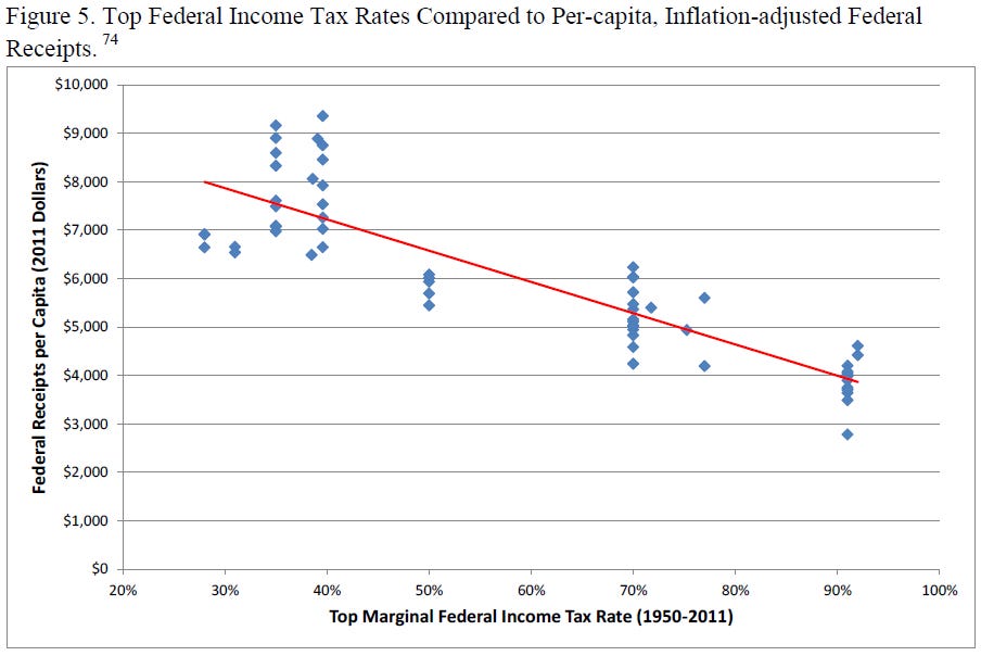
Figure 5 shows federal receipts per capita (adjusted for inflation) compared to the top federal marginal income tax rate. The data show a clear trend — in years in which the top income tax rate was higher, federal receipts were lower. It is possible that the data reveal the federal government’s response to tax receipts — when tax receipts are low, the federal government is compelled to raise rates in an attempt to raise revenue. One way to control for this effect is to compare the top income tax rate to federal receipts in future years.

Figure 6 shows the relationship between the top income tax rate and tax revenues per capita two years later. The same negative relationship appears. In fact, the negative relationship appears (with very little change in the slope) for federal receipts one, three, and four years into the future as well.

The same negative relationship appears for the top capital gains tax rate (figure 7) for the average effective corporate income tax rate (figure 8). One of the few positive relationships is between the average marginal income and payroll tax rates and federal receipts per capita (figure 9).

While history suggests that the government has far less ability to increase its revenue than politicians would have us believe, history also shows that the government has no difficulty increasing its spending. In 1950, the federal government spent $3,000 per person in today’s dollars. By 2010, that figure had risen to more than $12,000 (figure 9). In 60 years, the federal government’s spending on a per person and inflation-adjusted basis quadrupled.

However, if Keynesian theory held, we should also expect to see a positive relationship between government spending now and economic growth in the future.

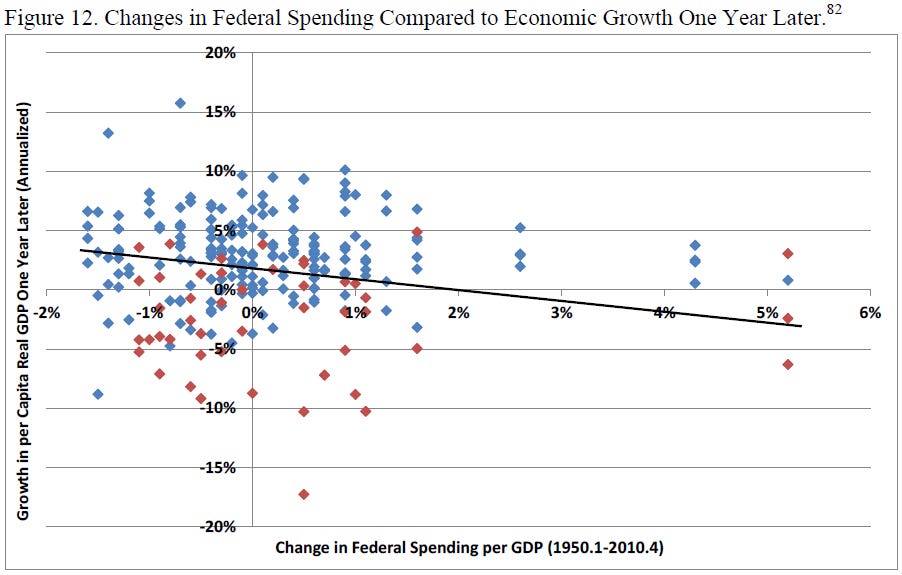
Reality does not reflect this theory. Figure 12 shows the relationship between changes in federal spending and real per capita economic growth one year in the future. The relationship appears to be negative, though it is statistically indistinguishable from a flat trend line.

It is possible that it takes more than a year for government spending to affect the economy. Comparing changes in federal spending to economic growth two years later reveals a slightly positive relationship, but again the relationship is statistically indistinguishable from a flat trend line (figure 13). Extending the time horizon out as far as 10 years reveals relationships between government spending and economic growth that are sometimes slightly positive (for 2-, 3-, and 9-year horizons) and sometimes slightly negative (for 1-, 4-, 5-, 6-, 7-, 8-, and 10-year horizons), but always statistically zero.

A counterargument is that what really matters is the relationship between stimulus spending and economic growth during recessions.

If we restrict our vision to recessions only (the red dots in figures 11–13), the same story emerges. There is no significant relationship between changes in government spending during recessions and economic growth at any point from one to 10 years later.

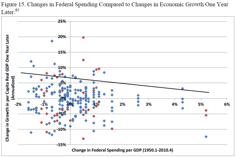
One could argue that because of a persistent baseline growth in per capita GDP, changes in federal spending should be compared to changes in per capita GDP growth. That comparison yields the same absence of results as do the previous comparisons. Figures 14 and 15 show the contemporaneous and one-year lagged relationships.

Although factors other than government spending influence economic growth, unless Keynesians are prepared to claim that those factors have conspired to counteract government spending on a consistent basis and over many decades, Keynesians are left having to explain why 60 years of economic data do not show, at least on average, economic growth accompanying increased government spending.

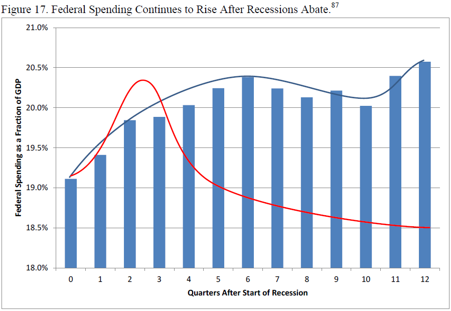
Figure 16 confirms the observation in figure 15 that stimulus spending is destabilizing because it continues to accelerate after the recession has begun to subside. It also confirms the suspicion among some economists that big government politicians do not believe in Keynes but judiciously quote him to justify expanding the government’s control over the economy.

5. Final Thoughts

The second hurdle is timing. Even if Keynesian theory were sound, if policy makers cannot time stimulus spending correctly, then their efforts will actually destabilize the economy by reducing spending during recessions and increasing spending during expansions. Evidence suggests not only that policy makers cannot get their timing right, but that this inability has been common knowledge among policy makers for decades.

The third hurdle is reversing the stimulus spending. Even if Keynesian theory were sound and even if policy makers could get the timing right, they would need the political will to shut off the stimulus spending at the ends of the recessions.

Since 1950, annual per capita real federal outlays have declined 23 times but increased 39 times, and each increase has been, on average, 2.5 times the size of each decrease.

Focusing on discretionary spending only produces a similar story. Since 1962, federal per capita real discretionary spending has increased 27 times but decreased only 22 times. On average, each increase was 1.34 times the size of each decrease.

An examination of 150 countries over 25 years shows that as economies grow, the optimal size of government — the government spending per dollar of GDP that is associated with maximum economic growth — declines. It may be that when a country is small, private investment is commensurately small, financial markets are less developed, and government can play a useful role in funding industries that require large start-up costs. This need would diminish as the country’s economy develops.

________________________________________________________________ ________________________________________________________________

John Maynard Keynes, toward the end of his life, wrote :

Organized public works, at home and abroad, may be the right cure for a chronic tendency to a deficiency of effective demand. But they are not capable of sufficiently rapid organisation (and above all cannot be reversed or undone at a later date), to be the most serviceable instrument for the prevention of the trade cycle.

This statement sounds like a confession and highlights the discrepancy between keynesian theory and empirical evidence.