Re-analysis of Jensen's study of Capron and Duyme adoption data

The french adoption study, by Capron & Duyme (1989, Table 2; 1996, Table 3), attempted to show that IQ can be improved by adoption. Their numbers displayed an IQ gain of 15 or even 20 points (WISC-R). Jensen (1997) analyzed Capron and Duyme adoption data (1996) with N=38, a study often cited by environmentalists as evidence against the hereditarian hypothesis. Jensen showed that the IQ difference owing to the adoption of children from low-SES parents by high-SES families is not g-loaded while at the same time the IQ difference owing to low-SES versus high-SES biological families loaded in fact on the g factor or PC1. Plus, the SES-difference of adopted families correlated at only 0.099 with SES-difference of biological families.

But then Nisbett, in Intelligence and How to Get It (2009, pp. 240-241, footnote 33), challenged Jensen. Too bad, neither Rushton & Jensen (2010, p. 19) nor James J. Lee (2009, p. 250) discussed this topic. Nisbett’s discussion is worth quoting in full :

Many things can be said about this. (1) The difference in factor loadings on g across WISC subtests is relatively slight, so the reanalysis does not much affect conclusions about the impact of adoption on intelligence. (2) More importantly, there is no difference at all in average g loadings between the subtests that show a big difference between high- and low-SES adoptive parents and their offspring and those that show little difference. Both loadings are .71 on average. (3) The fact that the subtests that most differentiate between biological parents and their offspring have higher g loadings than the subtests that differentiate least is almost entirely due to the fact that the Coding subtest, which has by far the lowest g loading, is one of the tests that does not differentiate much between high- and low-SES biological parents and their offspring. If Coding is left out, the g loadings for the former average .79 and for the latter average .69 - not much of a difference. (4) The WISC is a heavily verbally oriented test - that is, it measures mostly crystallized intelligence, and the g loadings differ primarily to the extent that they measure verbal ability as opposed to performance or fluid skills. (5) Jensen himself (1998) said that the purest measure of fluid g is the Raven Progressive Matrices test. If we examine fluid g as defined by subtest correlations with the Raven scores, we find that the correlation for biological parents and their offspring flips direction. It is now the test with the highest g loadings that differentiate least between high- and low-SES biological parents and their siblings. So the question as to whether the genetic effect is more reflective of differences in g than the environmental effect is entirely a matter of deciding which is the real g - fluid or crystallized. See Flynn (2000a) for a more detailed explanation of these points in the context of race differences in IQ. More important than any of these points is that the adopted children of upper-middle-class parents did far better in terms of academic achievement than did the adopted children of lower-class parents. The results of their school achievement tests were substantially better and they were far less likely to be put back a grade. And Jensen has in other contexts expressed the view that academic achievement is highly reflective of g. In any case, we care more about school achievement than about IQ.

Annoying is the fact that Nisbett does not give us a justifiable reason for excluding the Coding item. As for the other claims he made, it is difficulty for me to make sense of these. But I can say that the last sentence is obviously wrong. Academic achievement is indeed highly reflective of g, but improvement in academic performance does not necessarily imply equivalent increases in g, if g increased at all, insofar as they are not perfectly correlated, and that achievement tests are more malleable than IQ tests (Murray, 2005; Gottfredson, 2003).

Now we test Nisbett’s 3rd claim :

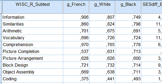
Above is the matrix displayed in Jensen (1997) for his PC analysis, that I copied in my SPSS data window; for details, see Jensen’s Table 2. Using these variables, I conduct a principal component analysis, as Jensen previously did, yielding the following SPSS output :

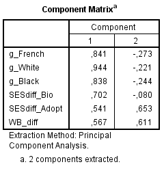
Now compare these figures with Jensen’s (1997) table 3. My numbers perfectly match Jensen’s numbers. My result does not appear to be a fluke. But because Nisbett considers the Coding subtest as being the problem, that is, the item to be removed, so then I removed that one and after running once again a PC analysis, I obtain those figures.

As we see, SESdiff_Adopt loaded equally well on PC1 and PC2, suggesting that IQ gains due to high-SES adopted families could be explained both by variance in g (0.541) and in non-g (0.653). Another difference is that the BW IQ differences now load equally well on PC1 (0.567) and PC2 (0.611). To note, the KMO and Bartlett’s Test shows a value of 0.55, with significance level of 0.164 after removing Coding, while the figures were intially 0.747 with significance level of 0.003. A high coefficient means that the patterns of correlations are relatively compact and that factor analysis should yield distinct and reliable factors. The congruence coefficients are displayed in my Excel sheet (here).

Remember the figures of g-loadings displayed in Jensen’s correlation matrix. The loadings are relatively high, and the Coding subtest is only about 0.375, 0.441, or 0.493. We get a range restriction problem if we remove this item, which is clearly not a smart idea. According to Jensen (1998, p. 382), it is recommended, among other things, that the variance of g-loadings is large enough for the method of correlated vectors to be used. Here’s a scatter plot, with and without Coding, of the correlation between SESdiff_Adopt and g_French, the Coding item being the black dot :

Indeed, the correlation between SESdiff_Adopt and g_French was null when using all subtests but became positive after removing Coding. But we also see that the presence of Coding is certainly not the primary responsible for the correlation between SESdiff_Bio and g_French. This is because there is a clear pattern in the SESdiff_Bio plot but no pattern at all in the SESdiff_Adopt plot. In any case, the data is not consistent with a purely environmental hypothesis.

There is another french adoption data. A paper by Duyme et al. (1999, Table 1) which is lauded as a proof against the hereditarian hypothesis. Again, they show substantial IQ gains (WISC-R=58, WAIS=7) in a sample of 65 deprived children, going from 7.7, 15.8 and 19.5 points for low, medium and high SES of adoptive parents. The authors concluded that IQ can be boosted with significant environmental changes. But there are issues. The IQ correlation before and after adoption is not much different from what is shown in the data of children who have not experienced an improvement in their environments (0.67 and 0.60 respectively). Furthermore, a sample of neglected children is hardly generalizable to the population at large. Finally, the SD of adopted children after adoption has become much larger, regardless of SES subgroup level, which suggests that the effect is extremely heterogeneous (e.g., some IQs went up, or down, or did not move) yet there is no causal mechanism proposed to explain this pattern.

The correlation of 0.67 between IQs before and after adoption is moderate and indicates a degree of stability close to the stability found in longitudinal studies of biological children who have not undergone an environmental change (r = 0.60 between 4 and 5 or 14 and 15 years of age) (41, 42).

Surely, this is not in line with what they expect or want us to believe. Even if the IQ gains appeared to be genuine IQ gains, that is, g gains, a large gain even by an amount of 20 points would not be inconsistent with the hereditarian model. Here’s what Herrnstein and Murray said, in The Bell Curve, pages 764 (fn.1) and 771 (fn.86) in my edition :

1. A brief refresher (see Chapter 4): A heritability of 60 percent (a mid-range estimate) says that 40 percent of the observed variation in intelligence would disappear if a magic wand wiped out the differences in those aspects of the environment that bear on intelligence. Given that variance is the standard deviation squared and that the standard deviation of IQ is 15, this means that 40 percent of 15² is due to environmental variation, which is to say that the variance would drop from 225 to 135 and the standard deviation would contract to 11.6 instead of 15 if all the environmental sources of variation disappeared.

86. A twenty-point swing is easily reconciled with a heritability of .6 for IQ. Suppose the high- and low-SES homes in the French studies represent the 90th and 10th centile of environmental quality, as the text says. A twenty-point swing in IQ from the 2d to the 98th centile of environmental quality would then imply that the standard deviation of home environment effects on IQ is 4.69. Squared, this means a variance of 22 attributable to home environment. But as we noted in note 1, a heritability of .6 implies that there is a variance of 225 - 135, or 90, attributable to environmental sources. The French adoption studies, in short, are consistent with the conclusion that about a quarter of environmental variance is the variance across homes (if our guesses about the adopting and biological home environments are not way off). Three-quarters of the environmental influence on intelligence must be uncorrelated with the family SES, according to the present analysis. Note again that the balance tips toward environmental factors outside families as being the more relevant than those provided by families in affecting IQ, as mentioned in Chapter 4.

Another recommended reading is Locurto (1990, pp. 287-289). Regardless, given the small sample sizes of these studies, it should be reckless to jump into quick conclusions. There are a lot more adoption data that need to be analyzed, and that I could have analyzed if researchers dared provide the data (email) instead of just saying “no we can’t” : an answer which I am now used to.

SPSS syntax :

FACTOR 
/VARIABLES g_French g_White g_Black SESdiff_Bio SESdiff_Adopt WB_diff 
/MISSING LISTWISE 
/ANALYSIS g_French g_White g_Black SESdiff_Bio SESdiff_Adopt WB_diff 
/PRINT UNIVARIATE INITIAL CORRELATION SIG DET KMO INV REPR AIC EXTRACTION 
/PLOT EIGEN 
/CRITERIA FACTORS(2) ITERATE(25) 
/EXTRACTION PC 
/ROTATION NOROTATE 
/METHOD=CORRELATION.