The Bell Curve: Intelligence and Class Structure in American Life, With a New Afterword by Charles Murray
The Bell Curve, 20 Years Later (Meng Hu's Blog)
Chapter 3 : The Economic Pressure to Partition
SPECIFICS SKILLS VERSUS G IN THE MILITARY … What explains how well they performed? For every one of the eighty-nine military schools, the answer was g – Charles Spearman’s general – intelligence. The correlations between g alone and military school grade ranged from an almost unbelievably high .90 for the course for a technical job in avionics repair down to .41 for that for a low-skill job associated with jet engine maintenance. [25] Most of the correlations were above .7. Overall, g accounted for almost 60 percent of the observed variation in school grades in the average military course, once the results were corrected for range restriction (the accompanying note spells out what it means to “account for 60 percent of the observed variation”). [26]
Did cognitive factors other than g matter at all? The answer is that the explanatory power of g was almost thirty times greater than of all other cognitive factors in ASVAB combined. The table below gives a sampling of the results from the eighty-nine specialties, to illustrate the two commanding findings: g alone explains an extraordinary proportion of training success; “everything else” in the test battery explained very little.
An even larger study, not quite as detailed, involving almost 350,000 men and women in 125 military specialties in all four armed services, confirmed the predominant influence of g and the relatively minor further predictive power of all the other factors extracted from ASVAB scores. [27] Still another study, of almost 25,000 air force personnel in thirty-seven different military courses, similarly found that the validity of individual ASVAB subtests in predicting the final technical school grades was highly correlated with the g loading of the subtest. [28]
TEST SCORES COMPARED TO OTHER PREDICTORS OF PRODUCTIVITY
How good a predictor of job productivity is a cognitive test score compared to a job interview? Reference checks? College transcript? The answer, probably surprising to many, is that the test score is a better predictor of job performance than any other single measure. This is the conclusion to be drawn from a meta-analysis on the different predictors of job performance, as shown in the table below.
The data used for this analysis were top heavy with higher-complexity jobs, yielding a higher-than-usual validity of .53 for test scores. However, even if we were to substitute the more conservative validity estimate of .4, the test score would remain the best predictor, though with close competition from biographical data. [41] The method that many people intuitively expect to be the most accurate, the job interview, has a poor record as a predictor of job performance, with a validity of only .14.
[...] The results in the table say, in effect, that among those choices that would be different, the employees chosen on the basis of test scores will on average be more productive than the employees chosen on the basis of any other single item of information.
Chapter 5 : Poverty
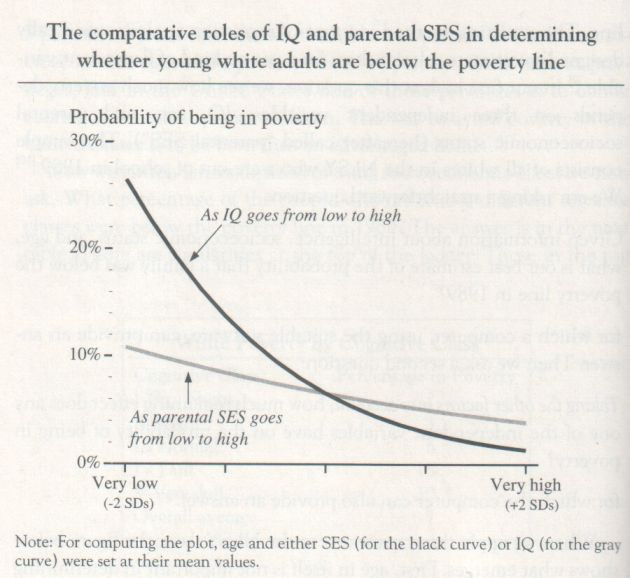
The black line lets you ask, “Imagine a person in the NLSY who comes from a family of exactly average socioeconomic background and exactly average age. [12] What are this person’s chances of being in poverty if he is very smart? Very dumb?” To find out his chances if he is smart, look toward the far right-hand part of the graph. A person with an IQ 2 SDs above the mean has an IQ of 130, which is higher than 98 percent of the population. Reading across to the vertical axis on the left, that person has less than a 2 percent chance of being in poverty (always assuming that his socioeconomic background was average). Now think about someone who is far below average in cognitive ability, with an IQ 2 SDs below the mean (an IQ of 70, higher than just 2 percent of the population). Look at the far left-hand part of the graph. Now, our imaginary person with an average socioeconomic background has about a 26 percent chance of being in poverty.
First, look at the pair of lines for the college graduates. We show them only for values greater than the mean, to avoid nonsensical implications (such as showing predicted poverty rate for a college graduate with an IQ two standard deviations below the mean). The basic lesson of the graph is that people who can complete a bachelor’s degree seldom end up poor, no matter what.
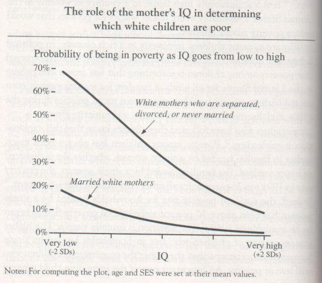
A married white woman with children who is markedly below average in cognitive ability – at the 16th centile, say, one standard deviation below the mean-from an average socioeconomic background had only a 10 percent probability of poverty.
The second point of the graph is that to be without a husband in the house is to run a high risk of poverty, even if the woman was raised in an average socioeconomic background. Such a woman, with even an average IQ, ran a 33 percent chance of being in poverty. If she was unlucky enough to have an IQ of only 85, she had more than a 50 percent chance – five times as high as the risk faced by a married woman of identical IQ and socioeconomic background. Even a woman with a conspicuously high IQ of 130 (two standard deviations above the mean) was predicted to have a poverty rate of 10 percent if she was a single mother, which is quite high compared to white women in general.
We used the same scale on the vertical axis in both of the preceding graphs to make the comparison with IQ easier. The conclusion is that no matter how rich and well educated the parents of the mother might have been, a separated, divorced, or never-married white woman with children and an average IQ was still looking at nearly a 30 percent chance of being below the poverty line, far above the usual level for whites and far above the level facing a woman of average socioeconomic background but superior IQ. We cannot even be sure that higher socioeconomic background reduces the poverty rate at all for unmarried women after the contribution of IQ has been extracted; the downward slope of the line plotted in the graph does not approach statistical significance. [20]
Chapter 6 : Schooling
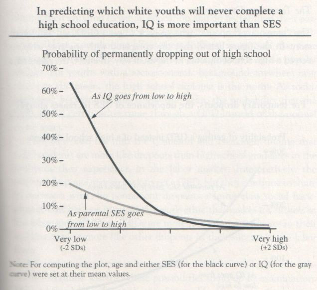
Of the whites who dropped out never to return, only three-tenths of 1 percent met a realistic definition of the gifted-but-disadvantaged dropout (top quartile of IQ, bottom quartile of socioeconomic background.)
In terms of this figure, a student with very well-placed parents, in the top 2 percent of the socioeconomic scale, had only a 40 percent chance of getting a college degree if he had only average intelligence. A student with parents of only average SES – lower middle class, probably without college degrees themselves – who is himself in the top 2 percent of IQ had more than a 75 percent chance of getting a degree.
Chapter 7 : Unemployment, Idleness, and Injury
Given equal age and IQ, a young man from a family with high socioeconomic status was more likely to spend time out of the labor force than the young man from a family with low socioeconomic status. [3] In contrast, IQ had a large positive impact on staying at work. A man of average age and socioeconomic background in the 2d centile of IQ had almost a 20 percent chance of spending at least a month out of the labor force, compared to only a 5 percent chance for a man at the 98th centile.
Chapter 8 : Family Matters
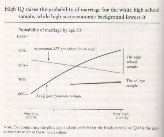
A high school graduate from an average socioeconomic background who was at the bottom of the IQ distribution (2 standard deviations below the mean) had a 60 percent chance of having married. A high school graduate at the top of the IQ distribution had an 89 percent chance of having married. Meanwhile, the independent role of socioeconomic status in the high school sample was either slightly negative or nil (the downward slope is not statistically significant).
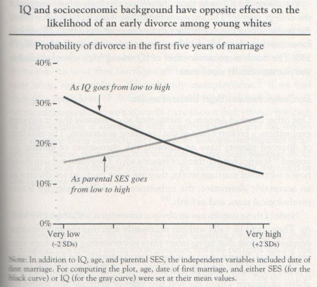
The consistent finding, represented fairly by the figure, was that higher IQ was still associated with a lower probability of divorce after extracting the effects of other variables, and parental SES had a significant positive relationship to divorce – that is, IQ being equal, children of higher-status families were more likely to get divorced than children of lower-status families. [10]
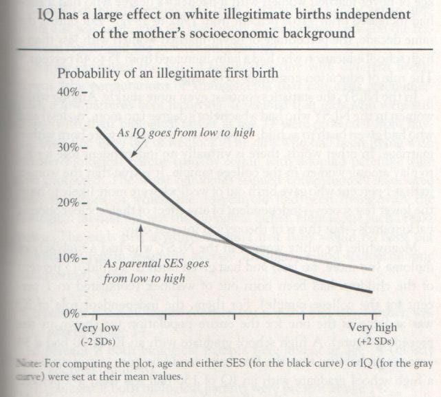
Higher social status reduces the chances of an illegitimate first baby from about 19 percent for a woman who came from a very low status family to about 8 percent for a woman from a very high status family, given that the woman has average intelligence. Let us compare that 11 percentage point swing with the effect of an equivalent shift in intelligence (given average socioeconomic background). [28] The odds of having an illegitimate first child drop from 34 percent for a very dull woman to about 4 percent for a very smart woman, a swing of 30 percentage points independent of any effect of socioeconomic status.
Chapter 9 : Welfare Dependency
If we want to understand the independent relationship between IQ and welfare, the standard analysis, using just age, IQ, and parental SES, is not going to tell us much. We have to get rid of the confounding effects of being poor and unwed. For that reason, the analysis that yielded the figure below extracted the effects of the marital status of the mother and whether she was below the poverty line in the year before birth, in addition to the usual three variables. The dependent variable is whether the mother received welfare benefits during the year after the birth of her first child. As the black line indicates, cognitive ability predicts going on welfare even after the effects of marital status and poverty have been extracted.
According to the figure, when it comes to chronic white welfare mothers, the independent effect of the young woman’s socioeconomic background is substantial. Whether it becomes more important than IQ as the figure suggests is doubtful (the corresponding analysis in Appendix 4 says no), but clearly the role of socioeconomic background is different for all welfare recipients and chronic ones.
Chapter 10 : Parenting
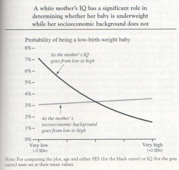
A low IQ is a major risk factor, whereas the mother’s socioeconomic background is irrelevant. A mother at the 2d centile of IQ had a 7 percent chance of giving birth to a low-birth-weight baby, while a mother at the 98th percentile had less than a 2 percent chance.
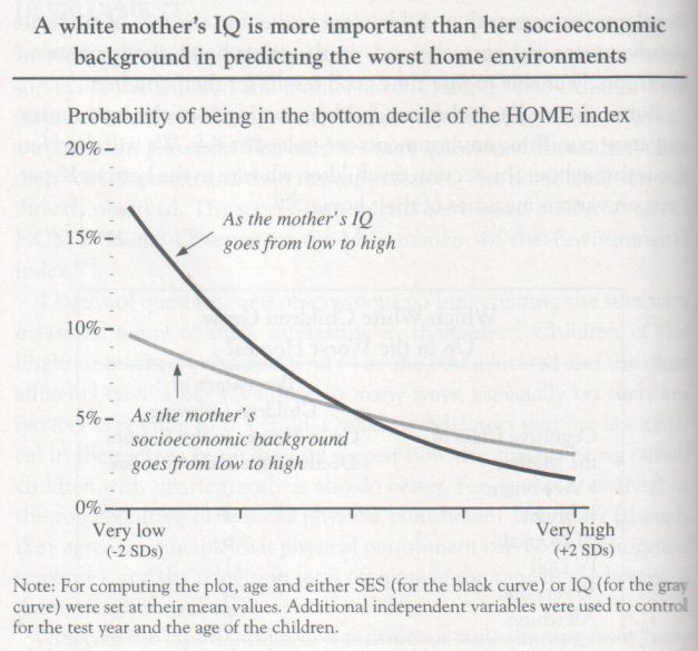
Both factors play a significant role, but once again it is worse (at least for the white NLSY population) to have a mother with a low IQ than one from a low socioeconomic background. Given just an average IQ for the mother, even a mother at the 2d centile on socioeconomic background had less than a 10 percent chance of providing one of the “worst homes” for her children. But even with average socioeconomic background, a mother at the 2d centile of intelligence had almost a 17 percent chance of providing one of these “worst homes.”
What independent role, if any, does the mother’s IQ have on the probability that her child experiences a substantial developmental problem? We created a simple “developmental problem index,” in which the child scores Yes if he or she were in the bottom decile of any of the four indicators in a given test year, and No if not. The results are shown in the next figure. … The pattern shown in the figure generally applies to the four development indicators separately: IQ has a somewhat larger independent effect than socioeconomic background, but of modest size and marginal statistical significance.
A white child’s IQ in the NLSY sample went up by 6.3 IQ points for each increase of one standard deviation in the mother’s IQ, compared to 1.7 points for each increase of one standard deviation in the mother’s socioeconomic background (in an analysis that also extracted the effects of the mother’s age, the test year, and the age of the child when tested). … A mother at the 2d IQ centile but of average socioeconomic background had a 30 percent chance that her child would be in the bottom decile of IQ, compared to only a 10 percent chance facing the woman from an equivalently terrible socioeconomic background (2d centile on the SES index) but with an average IQ.
Chapter 11 : Crime
DEPRAVED OR DEPRIVED?
When crime is changing quickly, it seems hard to blame changing personal characteristics rather than changing social conditions. But bear in mind that personal characteristics need not change everywhere in society for crime’s aggregate level in society to change. Consider age, for example, since crime is mainly the business of young people between 15 and 24. [6] When the age distribution of the population shifts toward more people in their peak years for crime, the average level of crime may be expected to rise. Or crime may rise disproportionately if a large bulge in the youthful sector of the population fosters a youth culture that relishes unconventionality over traditional adult values. The exploding crime rate of the 1960s is, for example, partly explained by the baby boomers’ reaching adolescence. [7] Or suppose that a style of child rearing sweeps the country, and it turns out that this style of child rearing leads to less control over the behavior of rebellious adolescents. The change in style of child rearing may predictably be followed, fifteen or so years later, by a change in crime rates. If, in short, circumstances tip toward crime, the change will show up most among those with the strongest tendencies to break laws (or the weakest tendencies to obey them). [8] …
Perhaps the link between crime and low IQ is even more direct. A lack of foresight, which is often associated with low IQ, raises the attractions of the immediate gains from crime and lowers the strength of the deterrents, which come later (if they come at all). To a person of low intelligence, the threats of apprehension and prison may fade to meaninglessness. They are too abstract, too far in the future, too uncertain.
Low IQ may be part of a broader complex of factors. An appetite for danger, a stronger-than-average hunger for the things that you can get only by stealing if you cannot buy them, an antipathy toward conventionality, an insensitivity to pain or to social ostracism, and a host of derangements of various sorts, combined with low IQ, may set the stage for a criminal career.
Finally, there are moral considerations. Perhaps the ethical principles for not committing crimes are less accessible (or less persuasive) to people of low intelligence. They find it harder to understand why robbing someone is wrong, find it harder to appreciate the values of civil and cooperative social life, and are accordingly less inhibited from acting in ways that are hurtful to other people and to the community at large.
THE LINK BETWEEN COGNITIVE ABILITY AND CRIMINAL BEHAVIOR: AN OVERVIEW
The Size of the IQ Gap
How big is the difference between criminals and the rest of us? Taking the literature as a whole, incarcerated offenders average an IQ of about 92, 8 points below the mean. The population of nonoffenders averages more than 100 points [...]
Do the Unintelligent Ones Commit More Crimes – or Just Get Caught More Often?
In the small amount of data available, the IQs of uncaught offenders are not measurably different from the ones who get caught. [26] Among those who have criminal records, there is still a significant negative correlation between IQ and frequency of offending. [27] Both of these kinds of evidence imply that differential arrests of people with varying IQs, assuming they exist, are a minor factor in the aggregate data.
Intelligence as a Preventative
One study followed a sample of almost 1,500 boys born in Copenhagen, Denmark, between 1936 and 1938. [28] Sons whose fathers had a prison record were almost six times as likely to have a prison record themselves (by the age of 34-36) as the sons of men who had no police record of any sort. Among these high-risk sons, the ones who had no police record at all had IQ scores one standard deviation higher than the sons who had a police record. [29]
The protective power of elevated intelligence also shows up in a New Zealand study. Boys and girls were divided on the basis of their behavior by the age of 5 into high and low risk for delinquency. High-risk children were more than twice as likely to become delinquent by their mid-teens as low-risk children. The high-risk boys or girls who did not become delinquent were the ones with the higher IQs. This was also true for the low-risk boys and girls: The nondelinquents had higher IQs than the delinquents. [30]
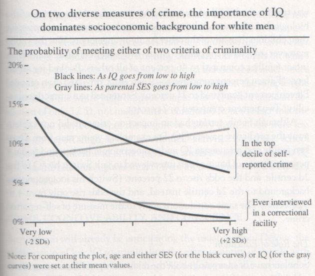
Both measures of criminality have weaknesses but different weaknesses. One relies on self-reports but has the virtue of including uncaught criminality; the other relies on the workings of the criminal justice system but has the virtue of identifying people who almost certainly have committed serious offenses. For both measures, after controlling for IQ, the men’s socioeconomic background had little or nothing to do with crime. In the case of the self-report data, higher socioeconomic status was associated with higher reported crime after controlling for IQ. In the case of incarceration, the role of socioeconomic background was close to nil after controlling for IQ, and statistically insignificant. By either measure of crime, a low IQ was a significant risk factor.
Chapter 12 : Civility and Citizenship
As intuition might suggest, “upbringing” in the form of socioeconomic background makes a significant difference. But for the NLSY sample, it was not as significant as intelligence. Even when we conduct our usual analyses with the education subsamples – thereby guaranteeing that everyone meets one of the criteria (finishing high school) – a significant independent role for IQ remains. Its magnitude is diminished for the high school sample but not, curiously, for the college sample. The independent role of socioeconomic background becomes insignificant in these analyses and, in the case of the high-school-only sample, goes the “wrong” way after cognitive ability is taken into account.
Chapter 13 : Ethnic Differences in Cognitive Ability
For practical purposes, environments are heritable too. The child who grows up in a punishing environment and thereby is intellectually stunted takes that deficit to the parenting of his children. The learning environment he encountered and the learning environment he provides for his children tend to be similar. The correlation between parents and children is just that: a statistical tendency for these things to be passed down, despite society’s attempts to change them, without any necessary genetic component. In trying to break these intergenerational links, even adoption at birth has its limits. Poor prenatal nutrition can stunt cognitive potential in ways that cannot be remedied after birth. Prenatal drug and alcohol abuse can stunt cognitive potential. These traits also run in families and communities and persist for generations, for reasons that have proved difficult to affect. [...]
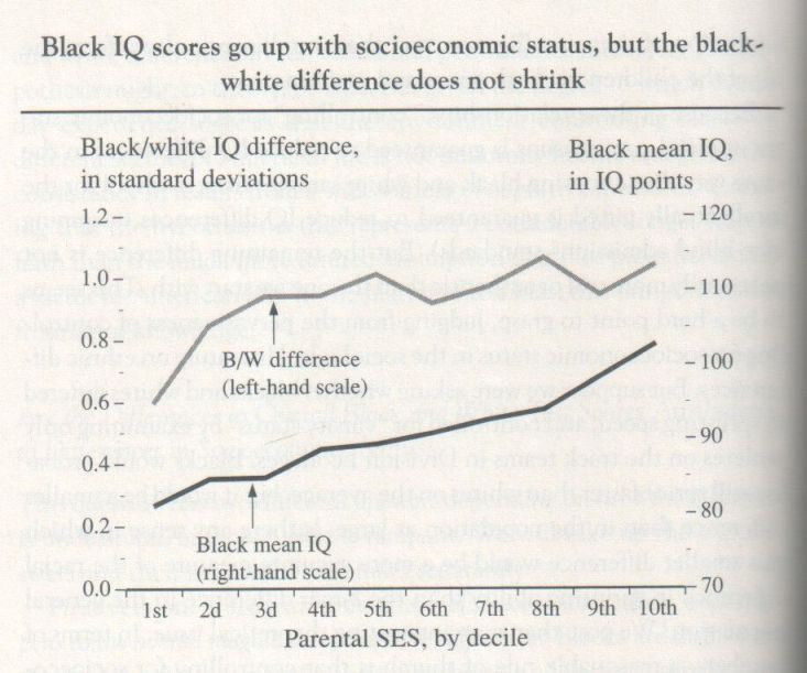
If you extract the effect of socioeconomic class, what happens to the overall magnitude of the B/W difference? … The NLSY gives a result typical of such analyses. The B/W difference in the NLSY is 1.21. In a regression equation in which both race and socioeconomic background are entered, the difference between whites and blacks shrinks to .76 standard deviation. [40] socioeconomic status explains 37 percent of the original B/W difference. This relationship is in line with the results from many other studies. [41]
The difficulty comes in interpreting what it means to “control” for socioeconomic status. … The trouble is that socioeconomic status is also a result of cognitive ability, as people of high and low cognitive ability move to correspondingly high and low places in the socioeconomic continuum.
IQ scores increase with economic status for both races. But as the figure shows, the magnitude of the B/W difference in standard deviations does not decrease. Indeed, it gets larger as people move up from the very bottom of the socioeconomic ladder. The pattern shown in the figure is consistent with many other major studies, except that the gap flattens out. In other studies, the gap has continued to increase throughout the range of socioeconomic status. [43]
Chapter 14 : Ethnic Inequalities in Relation to IQ
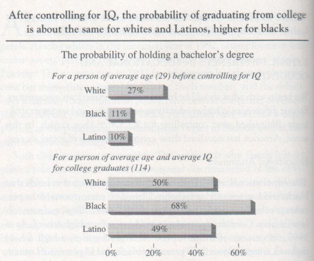
In this figure, the top three bars show that a white adult had a 27 percent chance of holding a bachelor’s degree, compared to the lower odds for blacks (11 percent) and Latinos (10 percent). The probabilities were computed through a logistic regression analysis. … The lower set of bars also presents the probabilities by ethnic group, but with one big difference: Now, the equation used to compute the probability assumes that each of these young adults has a certain IQ level. In this case, the computation assumes that everybody has the average IQ of all college graduates in the NLSY – a little over 114. We find that a 29-year-old (in 1990) with an IQ of 114 had a 50 percent chance of having graduated from college if white, 68 percent if black, and 49 percent if Latino. After taking IQ into account, blacks have a better record of earning college degrees than either whites or Latinos.
Before controlling for IQ and using unrounded figures, whites were almost twice as likely to be in high-IQ occupations as blacks and more than half again as likely as Latinos. [10] But after controlling for IQ, the picture reverses. The chance of entering a high-IQ occupation for a black with an IQ of 117 (which was the average IQ of all the people in these occupations in the NLSY sample) was over twice the proportion of whites with the same IQ. Latinos with an IQ of 117 had more than a 50 percent higher chance of entering a high-IQ occupation than whites with the same IQ. [11]
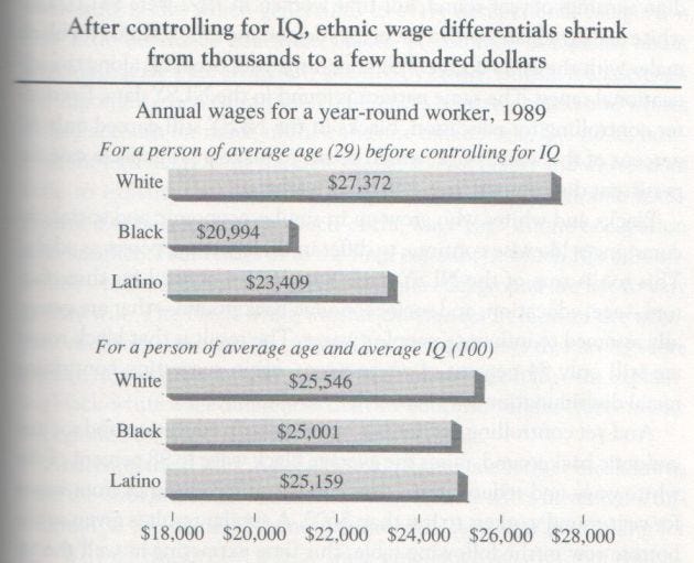
After controlling for IQ, the average black made 98 percent of the white wage. For Latinos, the ratio after controlling for IQ was also 98 percent of the white wage. Another way to summarize the outcome is that 91 percent of the raw black-white differential in wages and 90 percent of the raw Latino-white differential disappear after controlling for IQ.
A common complaint about wages is that they are artificially affected by credentialism. If credentials are important, then educational differences between blacks and whites should account for much of their income differences. The table, however, shows that knowing the educational level of blacks and whites does little to explain the difference in their wages. Socioeconomic background also fails to explain much of the wage gaps in one occupation after another. That brings us to the final column, in which IQs are controlled while education and socioeconomic background are left to vary as they will. The black-white income differences in most of the occupations shrink considerably. [...]
… When gender is added to the analysis, the black-white differences narrow by one or two additional percentage points for each of the comparisons. In the case of IQ, this means that the racial difference disappears altogether. Controlling for age, IQ, and gender (ignoring education and parental SES), the average wage for year-round black workers in the NLSY sample was 101 percent of the average white wage.
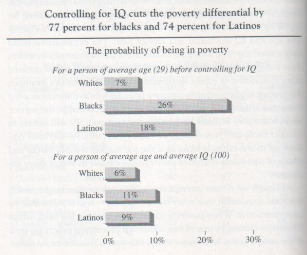
If commentators and public policy specialists were looking at a 6 percent poverty rate for whites against 11 percent for blacks – the rates for whites and blacks with IQs of 100 in the lower portion of the graphic – their conclusions might differ from what they are when they see the unadjusted rates of 7 percent and 26 percent in the upper portion. But even after controlling for IQ, the black poverty rate remains almost twice as high as the white rate – still a significant difference. [16]
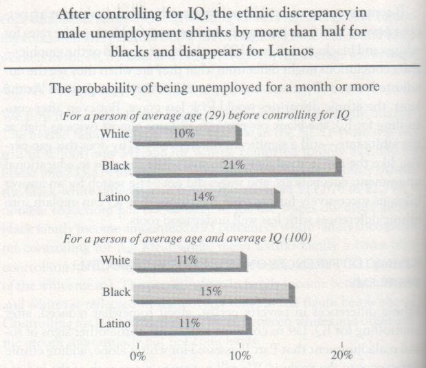
Dropping out of the labor force is similarly related to IQ. Controlling for IQ shrinks the disparity between blacks and whites by 65 percent and the disparity between Latinos and whites by 73 percent. [19]
As far as we are able to determine, this disparity cannot be explained away, no matter what variables are entered into the equation. … Controlling for IQ reduced the Latino-white difference by 44 percent but the black-white difference by only 20 percent. Nor does it change much when we add the other factors discussed in Chapter 8: socioeconomic background, poverty, coming from a broken home, or education.
Among white men, the proportion interviewed in a correctional facility after controlling for age was 2.4 percent; among black men, it was 13.1 percent. This large black-white difference was reduced by almost three-quarters when IQ was taken into account. The relationship of cognitive ability to criminal behavior among whites and blacks appears to be similar. [40]
Chapter 15 : The Demography of Intelligence
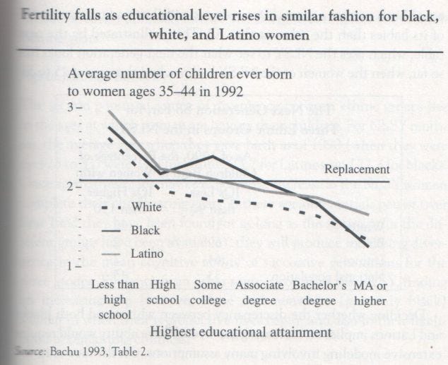
This figure represents almost total lifetime fertilities, and it tells a simple story. In all three groups of women, more education means lower fertility. The two minority groups have higher overall fertility, but not by much when education is taken into account. Given the known relationship between IQ and educational attainment, fertility is also falling with rising IQ for each ethnic group. Indeed, if one tries to look into this relationship by assigning IQ equivalents based on the relationship of educational attainment and cognitive ability in the NLSY, it appears that after equating for IQ, black women at a given IQ level may have lower fertility rates than either white or Latino women. [42]
Chapter 17 : Raising Cognitive Ability
There are a number of problems with this assumption. One basic error is to assume that new educational opportunities that successfully raise the average will also reduce differences in cognitive ability. Consider trying to raise the cognitive level by putting a public library in a community that does not have one. Adding the library could increase the average intellectual level, but it may also spread out the range of scores by adding points to the IQs of the library users, who are likely to have been at the upper end of the distribution to begin with. The literature on such « aptitude-treatment interactions » is large and complex. For example, providing computer assistance to a group of elementary school children learning arithmetic increased the gap between good and bad students; a similar effect was observed when computers were used to teach reading; the educational television program, « Sesame Street » increased the gap in academic performances between children from high- and low-status homes. These results do not mean that such interventions are useless for the students at the bottom, but one must be careful to understand what is and is not being improved: The performance of those at the bottom might improve, but they could end up even further behind their brighter classmates.
Raising IQ Among the School-Aged: Converging Results from Two Divergent Tries
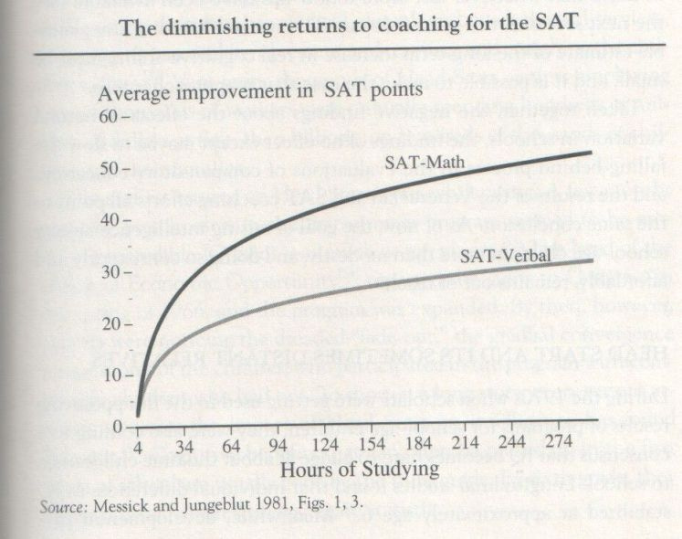
In the best of these analyses, Samuel Messick and Ann Jungeblut reviewed the published studies on coaching for the SAT, eliminated the ones that were methodologically unsound, and estimated in a regression analysis the point gain for a given number of hours spent studying for the test. [45] Their estimate of the effect of spending thirty hours on either the verbal or math test in a coaching course (including homework) was an average of sixteen points on the verbal SAT and twenty-five points for the math SAT. Larger investments in time earn larger payoffs with diminishing returns. For example, 100 hours of studying for either test earns an average twenty-four points on the verbal SAT and thirty-nine points on the math SAT. The next figure summarizes the results of their analysis.
Studying really does help, but consider what is involved. Sixty hours of work is not a trivial investment of time, but it buys (on average) only forty-one points on the combined Verbal and Math SATs – typically not enough to make much difference if a student is trying to impress an admissions committee. Even 300 hours – and now we are talking about two additional hours for 150 school days – can be expected to reap only seventy additional points on the combined score. And at 300 hours (150 for each test), the student is already at the flat part of the curve. Double the investment to 600 hours, and the expected gain is only fifteen more points.
Preschool Programs for Disadvantaged Children in General
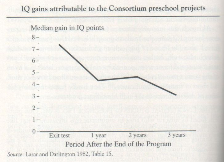
HEAD START. … Designed initially as a summer program, it was quickly converted into a year-long program providing classes for raising preschoolers’ intelligence and communication skills, giving their families medical, dental, and psychological services, encouraging parental involvement and training, and enriching the children’s diets. [52] Very soon, thousands of Head Start centers employing tens of thousands of workers were annually spending hundreds of millions of dollars at first, then billions, on hundreds of thousands of children and their families.
The earliest returns on Head Start were exhilarating. A few months spent by preschoolers in the first summer program seemed to be producing incredible IQ gains – as much as ten points. [53] … By then, however, experts were noticing the dreaded “fade-out,” the gradual convergence in test scores of the children who participated in the program with comparable children who had not. … Cognitive benefits that can often be picked up in the first grade of school are usually gone by the third grade. By sixth grade, they have vanished entirely in aggregate statistics.
PERRY PRESCHOOL. The study invoked most often as evidence that Head Start works is known as the Perry Preschool Program. David Weikart and his associates have drawn enormous media attention for their study of 123 black children … whose IQs measured between 70 and 85 when they were recruited in the early 1960s at the age of 3 or 4. [61] Fifty-eight children in the program received cognitive instruction five half-days [62] a week in a highly enriched preschool setting for one or two years, and their homes were visited by teachers weekly for further instruction of parents and children. The teacher-to-child ratio was high (about one to five), and most of the teachers had a master’s degree in appropriate child development and social work fields.
The fifty-eight children in the experimental group were compared with another sixty-five who served as the control group. By the end of their one or two years in the program, the children who went to preschool were scoring eleven points higher in IQ than the control group. But by the end of the second grade, they were just marginally ahead of the control group. By the end of the fourth grade, no significant difference in IQ remained. [63] Fadeout again.
Intensive Interventions for Children at Risk of Mental Retardation
THE ABECEDARIAN PROJECT. The Carolina Abecedarian Project started in the early 1970 … Through various social agencies, they located pregnant women whose children would be at high risk for retardation. … The program started when the babies were just over a month old, and it provided care for six to eight hours a day, five days a week, fifty weeks a year, emphasizing cognitive enrichment activities with teacher-to-child ratios of one to three for infants and one to four to one to six in later years, until the children reached the age of 5. It also included enriched nutrition and medical attention until the infants were 18 months old. [69]
… the major stumbling block to deciding what the Abecedarian Project has accomplished is that the experimental children had already outscored the controls on cognitive performance tests by at least as large a margin (in standard score units) by the age of 1 or 2 years, and perhaps even by 6 months, as they had after nearly five years of intensive day care. [71] There are two main explanations for this anomaly. Perhaps the intervention had achieved all its effects in the first months or the first year of the project … Or perhaps the experimental and control groups were different to begin with (the sample sizes for any of the experimental or control groups was no larger than fifteen and as small as nine, so random selection with such small numbers gives no guarantee that the experimental and control groups will be equivalent). To make things still more uncertain, test scores for children younger than 3 years are poor predictors of later intelligence test scores, and test results for infants at the age of 3 or 6 months are extremely unreliable. It would therefore be difficult in any case to assess the random placement from early test scores.
THE MILWAUKEE PROJECT. … The famous Milwaukee Project started in 1966 … Healthy babies of poor black mothers with IQs below 75 were almost, but not quite, randomly assigned to no day care at all or day care starting at 3 months and continuing until they went to school. … The families of the babies selected for day care received a variety of additional services and health care. The mothers were paid for participation, received training in parenting and job skills, and their other young children received free child care.
Soon after the Milwaukee project began, reports of enormous net gains in IQ (more than 25 points) started appearing in the popular media and in psychology textbooks. [72]
By the age of 12 to 14 years, the children who had been in the program were scoring about ten points higher in IQ than the controls. … But this increase was not accompanied by increases in school performance compared to the control group. Experimental and control groups were both one to two years retarded in reading and math skills by the time they reached fourth grade; their academic averages and their achievement scores were similar, and they were similarly rated by their teachers for academic competence. From such findings, psychologists Charles Locurto and Arthur Jensen have concluded that the program’s substantial and enduring gain in IQ has been produced by coaching the children so well on taking intelligence tests that their scores no longer measure intelligence or g very well. [75]
Appendix 1 : Statistics for People Who Are Sure They Can’t Learn Statistics
How Do You Compute a Standard Deviation?
Suppose that your high school class consisted of just two people who were 66 inches and 70 inches. Obviously, the average is 68 inches. Just as obviously, one person is 2 inches shorter than average, one person is 2 inches taller than average. The standard deviation is a kind of average of the differences from the mean – 2 inches, in this example. Suppose you add two more people to the class, one who is 64 inches and the other who is 72 inches. The mean hasn’t changed (the two new people balance each other off exactly). But the newcomers are each 4 inches different from the average height of 68 inches, so the standard deviation, which measures the spread, has gotten bigger as well. Now two people are 4 inches different from the average and two people are 2 inches different from the average. That adds up to a total 12 inches, divided among four persons. The simple average of these differences from the mean is 3 inches (12 / 4), which is almost (but not quite) what the standard deviation is. To be precise, the standard deviation is calculated by squaring the deviations from the mean, then summing them, then finding their average, then taking the square root of the result. In this example, two people are 4 inches from the mean and two are 2 inches from the mean. The sum of the squared deviations is 40 (16 + 16 + 4 + 4). Their average is 10 (40 / 4). And the square root of 10 is 3.16, which is the standard deviation for this example, The technical reasons for using the standard deviation instead of the simple average of the deviations from the mean are not necessary to go into, except that, in normal distributions, the standard deviation has wonderfully convenient properties. If you are looking for a short, easy way to think of a standard deviation, view it as the average difference from the mean.
As an example of how a standard deviation can be used to compare apples and oranges, suppose we are comparing the Olympic women’s gymnastics team and NBA basketball teams. You see a woman who is 5 feet 6 inches and a man who is 7 feet. You know from watching gymnastics on television that 5 feet 6 inches is tall for a woman gymnast, and 7 feet is tall even for a basketball player. But you want to do better than a general impression. Just how unusual is the woman, compared to the average gymnast on the U.S. women’s team, and how unusual is the man, compared to the average basketball player on the U.S. men’s team?
We gather data on height among all the women gymnasts, and determine that the mean is 5 feet 1 inches with a standard deviation (SD) of 2 inches. For the men basketball players, we find that the mean is 6 feet 6 inches and the SD is 4 inches. Thus the woman who is 5 feet 6 inches is 2.5 standard deviations taller than the average; the 7-foot man is only 1.5 standard deviations taller than the average. These numbers – 2.5 for the woman and 1.5 for the man – are called standard scores in statistical jargon. Now we have an explicit numerical way to compare how different the two people are from their respective averages, and we have a basis for concluding that the woman who is 5 feet 6 inches is a lot taller relative to other female Olympic gymnasts than a 7-foot man is relative to other NBA basketball players.
Appendix 4 : Regression Analyses from Part II
The size of R² tells something about the strength of the logistic relationship between the dependent variable and the set of independent variables, but it also depends on the composition of the sample, as do correlation coefficients in general. Even an inherently strong relationship can result in low values of R² if the data points are bunched in various ways, and relatively noisy relationships can result in high values if the sample includes disproportionate numbers of outliers. For example, one of the smallest R² in the following analyses, only 0.17, is for white men out of the labor force for four weeks or more in 1989. Apart from the distributional properties of the data that produce this low R², rough common-sense meaning to keep in mind is that the vast majority of NLSY white men were in the labor force even though they had low IQs or deprived socioeconomic backgrounds. But the parameter for zAFQT in that same equation is significant beyond the .001 level and large enough to make a big difference in the probability that a white male would be out of the labor force. This illustrates why we therefore consider the regression coefficients themselves (and their associated p values) to suit our analytic purposes better than R², and that is why those are the ones we relied on in the text.
Appendix 5 : Supplemental Material for Chapter 13
If for example, blacks do better in school than whites after choosing blacks and whites with equal test scores, we could say that the test was biased against blacks in academic prediction. Similarly, if they do better on the job after choosing blacks and whites with equal test scores, the test could be considered biased against blacks for predicting work performance. This way of demonstrating bias is tantamount to showing that the regression of outcomes on scores differs for the two groups. On a test biased against blacks, the regression intercept would be higher for blacks than whites, as illustrated in the graphic below. Test scores under these conditions would underestimate, or “underpredict,” the performance outcome of blacks. A randomly selected black and white with the same IQ (shown by the vertical broken line) would not have equal outcomes; the black would outperform the white (as shown by the horizontal broken lines). The test is therefore biased against blacks. On an unbiased test, the two regression lines would converge because they would have the same intercept (the point at which the regression line crosses the vertical axis).
But the graphic above captures only one of the many possible manifestations of predictive bias. Suppose, for example, a test was less valid for blacks than for whites. [1] In regression terms, this would translate into a smaller coefficient (slope in these graphics), which could, in turn, be associated either with or without a difference in the intercept. The next figure illustrates a few hypothetical possibilities.
All three black lines have the same low coefficient; they vary only in their intercepts. The gray line, representing whites, has a higher coefficient (therefore, the line is steeper). Begin with the lowest of the three black lines. Only at the very lowest predictor scores do blacks score higher than whites on the outcome measure. As the score on the predictor increases, whites with equivalent predictor scores have higher outcome scores. Here, the test bias is against whites, not blacks. For the intermediate black line, we would pick up evidence for test bias against blacks in the low range of test scores and bias against whites in the high range. The top black line, with the highest of the three intercepts, would accord with bias against blacks throughout the range, but diminishing in magnitude the higher the score.
Readers will quickly grasp that test scores can predict outcomes differently for members of different groups and that such differences may justify claims of test bias. So what are the facts? Do we see anything like the first of the two graphics in the data – a clear difference in intercepts, to the disadvantage of blacks taking the test? Or is the picture cloudier – a mixture of intercept and coefficient differences, yielding one sort of bias or another in different ranges of the test scores? When questions about data come up, cloudier and murkier is usually a safe bet. So let us start with the most relevant conclusion, and one about which there is virtual unanimity among students of the subject of predictive bias in testing: No one has found statistically reliable evidence of predictive bias against blacks, of the sort illustrated in the first graphic, in large, representative samples of blacks and whites, where cognitive ability tests are the predictor variable for educational achievement or job performance. In the notes, we list some of the larger aggregations of data and comprehensive analyses substantiating this conclusion. [2] We have found no modern, empirically based survey of the literature on test bias arguing that tests are predictively biased against blacks, although we have looked for them.
When we turn to the hundreds of smaller studies that have accumulated in the literature, we find examples of varying regression coefficients and intercepts, and predictive validities. This is a fundamental reason for focusing on syntheses of the literature. Smaller or unrepresentative individual studies may occasionally find test bias because of the statistical distortions that plague them. There are, for example, sampling and measurement errors, errors of recording, transcribing, and computing data, restrictions of range in both the predictor and outcome measurements, and predictor or outcome scales that are less valid than they might have been. [3] Given all the distorting sources of variation, lack of agreement across studies is the rule. [...]
Insofar as the many individual studies show a pattern at all, it points to overprediction for blacks. More simply, this body of evidence suggests that IQ tests are biased in favor of blacks, not against them. The single most massive set of data bearing on this issue is the national sample of more than 645,000 school children conducted by sociologist James Coleman and his associates for their landmark examination of the American educational system in the mid-1960s. Coleman’s survey included a standardized test of verbal and nonverbal IQ, using the kinds of items that characterize the classic IQ test and are commonly thought to be culturally biased against blacks: picture vocabulary, sentence completion, analogies, and the like. The Coleman survey also included educational achievement measures of reading level and math level that are thought to be straightforward measures of what the student has learned. If IQ item are culturally biased against blacks, it could be predicted that a black student would do better on the achievement measures than the putative IQ measure would lead one to expect (this is the rationale behind the current popularity of steps to modify the SAT so that it focuses less on aptitude and more on measures of what has been learned). But the opposite occurred. Overall, black IQ scores overpredicted black academic achievement by .26 standard deviations. [6] …
A second major source of data suggesting that standardized tests overpredict black performance is the SAT. Colleges commonly compare the performance of freshmen, measured by grade point average, against the expectations of their performance as predicted by SAT scores. A literature review of studies that broke down these data by ethnic group revealed that SAT scores overpredicted freshman grades for blacks in fourteen of fifteen studies, by a median of .20 standard deviation. [7] In five additional studies where the ethnic classification was “minority” rather than specifically “black,” the SAT score overpredicted college performance in all five cases, by a median of .40 standard deviation. [8]
For job performance, the most thorough analysis is provided by the Hartigan Report, assessing the relationship between the General Aptitude Test Battery (GATB) and job performance measures. Out of seventy-two studies that were assembled for review, the white intercept was higher than the black intercept in sixty of them – that is, the GATB overpredicted black performance in sixty out of the seventy-two studies. [9] Of the twenty studies in which the intercepts were statistically significantly different (at the .01 level), the white intercept was greater than the black intercept in all twenty cases. [10]
These findings about overprediction apply to the ordinary outcome measures of academic and job performance. But it should also be noted that “overprediction” can be a misleading concept when it is applied to outcome measures for which the predictor (IQ, in our continuing example) has very low validity. Inasmuch as blacks and whites differ on average in their scores on some outcome that is not linked to the predictor, the more biased it will be against whites. Consider the next figure, constructed on the assumption that the predictor is nearly invalid and that the two groups differ on average in their outcome levels.
This situation is relevant to some of the outcome measures discussed in Chapter 14, such as short-term male unemployment, where the black and white means are quite different, but IQ has little relationship to short-term unemployment for either whites or blacks. This figure was constructed assuming only that there are factors influencing outcomes that are not captured by the predictor, hence its low validity, resulting in the low slope of the parallel regression lines. [11] The intercepts differ, expressing the generally higher level of performance by whites compared to blacks that is unexplained by the predictor variable. If we knew what the missing predictive factors are, we could include them in the predictor, and the intercept difference would vanish – and so would the implication that the newly constituted predictor is biased against whites. What such results seem to be telling us is, first, that IQ tests are not predictively biased against blacks but, second, that IQ tests alone do not explain the observed black-white differences in outcomes. It therefore often looks as if the IQ test is biased against whites.
Appendix 3 : Technical Issues Regarding the Armed Forces Qualification Test as a Measure of IQ
Years of Education and the AFQT Score
For the AFQT as for other IQ tests, scores vary directly with educational attainment, leaving aside for the moment the magnitude of reciprocal cause and effect. But to what extent could we expect that, if we managed to keep low-scoring students in school for another year or two, their AFQT scores would have risen appreciably?
Chapter 17 laid out the general answer from a large body of research: Systematic attempts to raise IQ through education (exemplified by the Venezuelan experiment and the analyses of SAT coaching) can indeed have an effect on the order of .2 standard deviation, or three IQ points. As far as anyone can tell, there are diminishing marginal benefits of this kind of coaching (taking three intensive SAT coaching programs in succession will raise a score by less than three times the original increment).
We may explore the issue more directly by making use of the other IQ scores obtained for members of the NLSY. Given scores that were obtained several years earlier than the AFQT score, to what extent do the intervening years of education appear to have elevated the AFQT!
Underlying the discussion is a simple model:
The earlier IQ score affects both years of education and is a measure of the same thing that AFQT measures. Meanwhile, the years of education add something (we hypothesize) to the AFQT score that would not otherwise have been added.
Actually testing the model means bringing in several complications, however. The elapsed time between the earlier IQ test and the AFQT test presumably affects the relationships. So does the age of the subject (a subject who took the test at age 22 had a much different “chance” to add years of education than did a subject who took the test at age 18, for example). The age at which the earlier IQ test was taken is also relevant, since IQ test scores are known to become more stable at around the age of 6. But the main point of the exercise may be illustrated straightforwardly. We will leave the elaboration to our colleagues.
The database consists of all NLSY students who had an earlier IQ test score, as reported in the table on page 596, plus students with valid Stanford-Binet and WISC scores (too few to report separately). We report the results for two models in the table below, with the AFQT score as the dependent variable in both cases. In the first model, the explanatory variables are the earlier IQ score, age at the first test, elapsed years between the two tests, and type of test (entered as a vector of dummy variables). In the second model, we add years of education as an independent variable. An additional year of education is associated with a gain of 2.3 centiles per year, in line with other analyses of the effects of education on IQ. [17] What happens if the dependent variable is expressed in standardized scores rather than percentiles? In that case (using the same independent variables), the independent effect of education is to increase the AFQT score by .07 standard deviation, or the equivalent of about one IQ point per year – also in line with other analyses.
We caution against interpreting these coefficients literally across the entire educational range. Whereas it may be reasonable to think about IQ gains for six additional years of education when comparing subjects who had no schooling versus those who reached sixth grade, or even comparing those who dropped out in sixth grade and those who remained through high school, interpreting these coefficients becomes problematic when moving into post-high school education.
The negative coefficient for “elapsed years between tests” in the table above is worth mentioning. Suppose that the true independent relationship between years of education and AFQT is negatively accelerated – that is, the causal importance of the elementary grades in developing a person’s IQ is greater than the causal role of, say, graduate school. If so, then the more years of separation between tests, the lower would be the true value of the dependent variable, AFQT, compared to the predicted value in a linear regression, because people with many years of separation between tests in the sample are, on average, getting less incremental benefit of years of education than the sample with just a few years of separation. The observed results are consistent with this hypothesis.


