Here, I will explain how to use the so-called "Yhat" or predicted values of Y when doing regression (OLS, logistic and multilevel).
(Update 2017) This article is based on my paper: Hu, M. (2017). An update on the secular narrowing of the Black-White gap in the Wordsum vocabulary test (1974-2012). Mankind Quarterly, 58(2), 324-354.
I recommend to download my subset of the GSS data : https://osf.io/hiuzk/. The syntax I am using here is for Stata and SPSS. If you don't have either of these softwares, you may want to use the free software R. You have to read my introduction to R for advanced statistics and use my R syntax if you want to reproduce the analyses below.
The results are identical between the softwares but not for sample sizes. This is because when sampling weight is used, Stata continues to treat N as observed sample size while SPSS treats N as weighted sample size.
For the creation of the relevant variables, here's Stata :
keep if age<70
gen weight = wtssall*oversamp
gen gender = sex-1
gen bw = 0 if race==2
replace bw = 1 if race==1
replace bw = . if missing(race)
gen blackwhite2000after=1 if year>=2000 & race==1 & hispanic==1
replace blackwhite2000after=0 if year>=2000 & race==2 & hispanic==1
gen blackwhite2000before=1 if year<2000 & race==1
replace blackwhite2000before=0 if year<2000 & race==2
gen bw1 = max(blackwhite2000after,blackwhite2000before)
replace wordsum = . if wordsum<0
replace wordsum = . if wordsum>10
gen bw1wordsum = bw1*wordsum
gen income = realinc
replace income = . if income==0
gen logincome = log(income)
gen logincomec = logincome-10.13
replace educ = . if educ>20
replace degree = . if degree>4
gen educc = educ-13.09
gen degreec = degree-1.39
gen agec = age-40.62
gen agec2 = agec^2
gen agec3 = agec^3
gen bw1agec = bw1*agec
gen bw1agec2 = bw1*agec2
gen bw1agec3 = bw1*agec3
gen cohortc = cohort-1952
gen cohortc2 = cohortc^2
gen cohortc3 = cohortc^3
gen cohortc4 = cohortc^4
gen cohortc5 = cohortc^5
gen bw1cohortc = bw1*cohortc
gen bw1cohortc2 = bw1*cohortc2
gen bw1cohortc3 = bw1*cohortc3
gen bw1cohortc4 = bw1*cohortc4
gen bw1cohortc5 = bw1*cohortc5
recode age (18/26=1) (27/35=2) (36/44=3) (45/55=4) (56/69=5), generate(agegroup)
tabulate agegroup, gen(agedummy)
recode cohort (1905/1928=0) (1929/1943=1) (1944/1953=2) (1954/1962=3) (1963/1973=4) (1974/1994=5), generate(cohort6)
replace cohort6 = . if cohort6>5
tabulate cohort6, gen(cohortdummy)
gen bw1C1 = bw1*cohortdummy1
gen bw1C2 = bw1*cohortdummy2
gen bw1C3 = bw1*cohortdummy3
gen bw1C4 = bw1*cohortdummy4
gen bw1C5 = bw1*cohortdummy5
gen bw1C6 = bw1*cohortdummy6
recode cohort (1905/1915=0) (1916/1920=1) (1921/1925=2) (1926/1929=3) (1930/1933=4) (1934/1937=5) (1938/1941=6) (1942/1944=7) (1945/1947=8) (1948/1950=9) (1951/1953=10) (1954/1956=11) (1957/1959=12) (1960/1962=13) (1963/1965=14) (1966/1968=15) (1969/1972=16) (1973/1976=17) (1977/1980=18) (1981/1985=19) (1986/1994=20), generate(cohort21)
replace cohort21 = . if cohort21>20
recode age (18/23=1) (24/28=2) (29/33=3) (34/38=4) (39/44=5) (45/50=6) (51/56=7) (57/62=8) (63/69=9), generate(age9)
tabulate age9, gen(aged)
gen bw1aged1 = bw1*aged1
gen bw1aged2 = bw1*aged2
gen bw1aged3 = bw1*aged3
gen bw1aged4 = bw1*aged4
gen bw1aged5 = bw1*aged5
gen bw1aged6 = bw1*aged6
gen bw1aged7 = bw1*aged7
gen bw1aged8 = bw1*aged8
gen bw1aged9 = bw1*aged9
replace worda = . if worda<0
replace worda = 0 if worda==9
replace wordb = . if wordb<0
replace wordb = 0 if wordb==9
replace wordc = . if wordc<0
replace wordc = 0 if wordc==9
replace wordd = . if wordd<0
replace wordd = 0 if wordd==9
replace worde = . if worde<0
replace worde = 0 if worde==9
replace wordf = . if wordf<0
replace wordf = 0 if wordf==9
replace wordg = . if wordg<0
replace wordg = 0 if wordg==9
replace wordh = . if wordh<0
replace wordh = 0 if wordh==9
replace wordi = . if wordi<0
replace wordi = 0 if wordi==9
replace wordj = . if wordj<0
replace wordj = 0 if wordj==9
keep if !missing(bw1)
keep if !missing(wordsum)
And here's SPSS :
DATASET NAME DataSet1 WINDOW=FRONT.
DATASET COPY DataSet2 WINDOW=FRONT.
DATASET ACTIVATE DataSet2.
SELECT if age<70.
EXECUTE.
set mxcells=9000.
compute weight = wtssall*oversamp.
RECODE wordsum (-1=SYSMIS) (99=SYSMIS).
RECODE worda (9=0) (-1=SYSMIS).
RECODE wordb (9=0) (-1=SYSMIS).
RECODE wordc (9=0) (-1=SYSMIS).
RECODE wordd (9=0) (-1=SYSMIS).
RECODE worde (9=0) (-1=SYSMIS).
RECODE wordf (9=0) (-1=SYSMIS).
RECODE wordg (9=0) (-1=SYSMIS).
RECODE wordh (9=0) (-1=SYSMIS).
RECODE wordi (9=0) (-1=SYSMIS).
RECODE wordj (9=0) (-1=SYSMIS).
RECODE race (2=0) (1=1) (else=sysmis) INTO bw.
DO IF (year>=2000 and race=1 and hispanic=1).
COMPUTE blackwhite2000after=1.
ELSE IF (year>=2000 and race=2 and hispanic=1).
COMPUTE blackwhite2000after=0.
END IF.
DO IF (year<2000 & race=1).
COMPUTE blackwhite2000before=1.
ELSE IF (year<2000 & race=2).
COMPUTE blackwhite2000before=0.
END IF.
COMPUTE bw1=SUM(blackwhite2000after, blackwhite2000before).
VALUE LABELS bw1 0 'black' 1 'white'.
COMPUTE bw1wordsum = bw1*wordsum.
RECODE realinc (0=SYSMIS).
COMPUTE logincome = ln(realinc).
COMPUTE logincomec = logincome-10.13.
RECODE educ (21 thru highest=sysmis).
RECODE degree (5 thru highest=sysmis).
COMPUTE educc = educ-13.09.
COMPUTE degreec = degree-1.39.
COMPUTE gender=sex-1.
COMPUTE agec=age-40.62.
COMPUTE agec2=agec**2.
COMPUTE agec3=agec**3.
COMPUTE bw1agec=bw1*agec.
COMPUTE bw1agec2=bw1*agec2.
COMPUTE bw1agec3=bw1*agec3.
COMPUTE cohortc = cohort-1952.
COMPUTE cohortc2 = cohortc**2.
COMPUTE cohortc3 = cohortc**3.
COMPUTE cohortc4 = cohortc**4.
COMPUTE cohortc5 = cohortc**5.
COMPUTE bw1cohortc = bw1*cohortc.
COMPUTE bw1cohortc2 = bw1*cohortc2.
COMPUTE bw1cohortc3 = bw1*cohortc3.
COMPUTE bw1cohortc4 = bw1*cohortc4.
COMPUTE bw1cohortc5 = bw1*cohortc5.
RECODE age (18 thru 26=1) (else=0) INTO agedummy1.
RECODE age (27 thru 35=1) (else=0) INTO agedummy2.
RECODE age (36 thru 44=1) (else=0) INTO agedummy3.
RECODE age (45 thru 55=1) (else=0) INTO agedummy4.
RECODE age (56 thru 69=1) (else=0) INTO agedummy5.
RECODE cohort (1905 thru 1928=1) (else=0) INTO cohortdummy1.
RECODE cohort (1929 thru 1943=1) (else=0) INTO cohortdummy2.
RECODE cohort (1944 thru 1953=1) (else=0) INTO cohortdummy3.
RECODE cohort (1954 thru 1962=1) (else=0) INTO cohortdummy4.
RECODE cohort (1963 thru 1973=1) (else=0) INTO cohortdummy5.
RECODE cohort (1974 thru 1994=1) (else=0) INTO cohortdummy6.
compute bw1C1 = bw1*cohortdummy1.
compute bw1C2 = bw1*cohortdummy2.
compute bw1C3 = bw1*cohortdummy3.
compute bw1C4 = bw1*cohortdummy4.
compute bw1C5 = bw1*cohortdummy5.
compute bw1C6 = bw1*cohortdummy6.
RECODE cohort (1905 thru 1915=0) (1916 thru 1920=1) (1921 thru 1925=2) (1926 thru 1929=3) (1930 thru 1933=4) (1934 thru 1937=5) (1938 thru 1941=6) (1942 thru 1944=7) (1945 thru 1947=8) (1948 thru 1950=9) (1951 thru 1953=10) (1954 thru 1956=11) (1957 thru 1959=12) (1960 thru 1962=13) (1963 thru 1965=14) (1966 thru 1968=15) (1969 thru 1972=16) (1973 thru 1976=17) (1977 thru 1980=18) (1981 thru 1985=19) (1986 thru 1994=20) (ELSE=SYSMIS) INTO cohort21.
RECODE age (18 thru 23=1) (24 thru 28=2) (29 thru 33=3) (34 thru 38=4) (39 thru 44=5) (45 thru 50=6) (51 thru 56=7) (57 thru 62=8) (63 thru 69=9) INTO age9.
recode age (18 thru 23=1) (else=0) into aged1.
recode age (24 thru 28=1) (else=0) into aged2.
recode age (29 thru 33=1) (else=0) into aged3.
recode age (34 thru 38=1) (else=0) into aged4.
recode age (39 thru 44=1) (else=0) into aged5.
recode age (45 thru 50=1) (else=0) into aged6.
recode age (51 thru 56=1) (else=0) into aged7.
recode age (57 thru 62=1) (else=0) into aged8.
recode age (63 thru 69=1) (else=0) into aged9.
compute bw1aged1 = bw1*aged1.
compute bw1aged2 = bw1*aged2.
compute bw1aged3 = bw1*aged3.
compute bw1aged4 = bw1*aged4.
compute bw1aged5 = bw1*aged5.
compute bw1aged6 = bw1*aged6.
compute bw1aged7 = bw1*aged7.
compute bw1aged8 = bw1*aged8.
compute bw1aged9 = bw1*aged9.
SELECT IF(NOT MISSING(wordsum)) and (NOT MISSING(bw1)).
EXECUTE.
WEIGHT BY weight.
The attentive reader would have noticed that I have dropped all observations having missing data on either wordsum or bw1. This is because most (if not all) softwares are flatly stupid. When we compute the predicted Y, or Yhat, the software will compute these values even for the observations that weren't included in the regression model. Let's say age variable has 50118 cases and my wordsum variable has 23817 cases. Also, assume that everyone having data on wordsum also has data on age. Listwise deletion employed in regression techniques will keep only 23817 cases. But what will happen is that Yhat will be computed for 50118 observations, just because age has 50118 observations. For what I have seen, it does not bias the computed values, but it adds some useless and fictitious values for the observations removed by the listwise deletion procedure. We do not want these additional values.
Mean-centering
Here, one question must be answered. Why am I using mean-centering ? Or, at least, center at any other value ? This is because the intercept is the value of Y predicted by the regression model (Yhat) when all independent X variables are equal to zero. The minimum age of the sample is 18. That implies the value 0 is not an observable value in my variable. So, if I use the original variable of age, my Yhat variable will be the wordsum score when people are aged 0. This obviously makes little sense. If wordsum increases with age, then, using the original variable of age will cause the values of Yhat to be too low. The value zero must be an observable value in all of the independent variables.
The other advantage of mean-centering is to avoid extreme multicollinearity. Multicollinearity is a trouble because interaction terms and squared/cubic terms are usually known to have an extremely high correlation with the main effect variables. When it happens, the software will typically remove the sources of that collinearity, and several variables will be dropped from the analysis.
Descriptive analysis
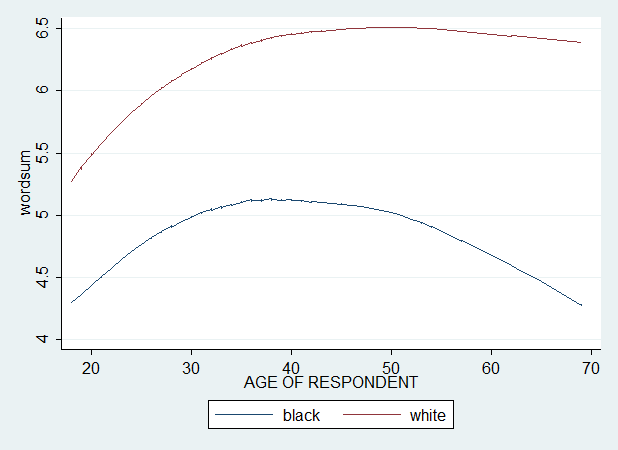
Before using regression, let's request a scatter plot of wordsum against age, by race. This is simply a descriptive analysis, but will reveal useful for reasons explained later.
In Stata, we do :
twoway (scatter wordsum cohort, msymbol(Oh) jitter(0)) (lowess wordsum cohort if bw1==0) (lowess wordsum cohort if bw1==1), ytitle(wordsum) legend(order(2 "black" 3 "white"))
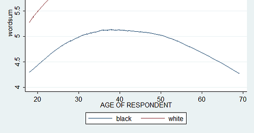
twoway (lowess wordsum age if bw1==0) (lowess wordsum age if bw1==1), ytitle(wordsum) legend(order(1 "black" 2 "white"))
In SPSS, we do :
GRAPH
/SCATTERPLOT(BIVAR)=cohort WITH wordsum BY bw1
/MISSING=LISTWISE
/SUBTITLE='Wordsum score across age by race'.
We want a loess curve, not a fitted line. In SPSS, it's a bother. There is no possibility to obtain fitted lines with syntax. We must edit the graph manually (properties -> loess -> apply). But anyway...
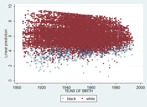
Usually, when we do scatter, we have a cloud of data points. This is because the analysis is a random effects approach. We didn't request or compute a fitted regression line. However, we can request a loess curve without scatter dots. This makes the graph easier to read. Because otherwise, we would have something like this :
In any case, there is a large black-white gap narrowing, which seems to have stopped quite recently. And we see that the gap widens considerably with age.
At this point, one may ask a question. Why using statistical modeling when a simple descriptive analysis already answered our question ?
What is modeling ?
To answer this question is to know first how Yhat is computed :
Yhat = intercept + coefficient*var1 + coefficient*var2 + coefficient*var3 ...
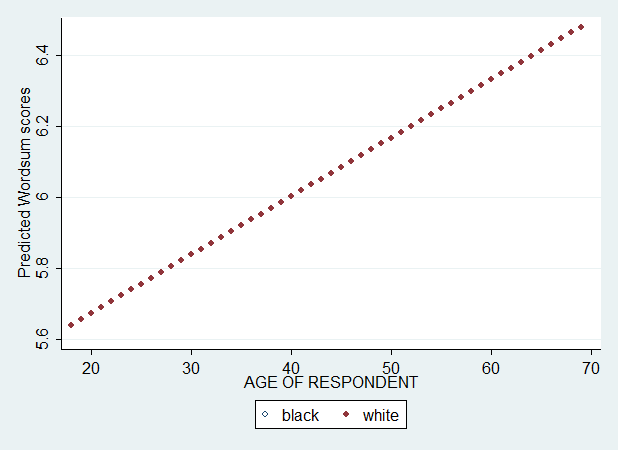
Let's say var1 is age, var2 is race, and var3 is age*race interaction. We first use a model with only age in independent (X) variable. After running this model, I save the predicted value (Yhat) and plot the Yhat against age by race.
Hm... What happened ? There is only one regression line. Ok. But, the reason is simple. The difference is that the first plot is a summary/descriptive analysis while this plot here is about modeling. In our regression, only age has been included. In other words, wordsum is allowed to vary only across ages. But not across races.
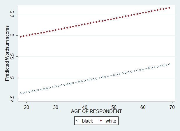
We have two separate lines, but they are parallel. We didn't include the interaction between age and race and, so, race difference was not allowed to vary across ages.
Now, I specify age, race, and age*race in my set of independent (X) variables.
This time, we get two separate regression lines and two separate slopes because our regression equation allows age effects to differ across races. If we have ignored the interaction, we would get two separate lines that are perfectly parallel. But even with this interaction, these lines are straight lines. As we have seen in the descriptive loess plot, the changes in wordsum score with age is not linear. Let's add age^2 and race*age^2.
In Stata, we do :
regress wordsum bw1 agec agec2 bw1agec bw1agec2 [pweight = weight], beta
predict wordsumpredictedage if e(sample), xb
label variable wordsumpredictedage "Predicted Wordsum scores"
graph twoway (scatter wordsumpredictedage age if bw1==0, msymbol(Oh)) (scatter wordsumpredictedage age if bw1==1, msymbol(O)), legend(label(1 black) label(2 white))
In SPSS, we do :
REGRESSION
/DESCRIPTIVES MEAN STDDEV CORR SIG N
/MISSING LISTWISE
/STATISTICS COEFF OUTS CI(95) R ANOVA COLLIN TOL CHANGE ZPP
/CRITERIA=PIN(.05) POUT(.10)
/NOORIGIN
/DEPENDENT wordsum
/METHOD=ENTER bw1 agec agec2 bw1agec bw1agec2
/SAVE PRED ZPRED.
GRAPH
/SCATTERPLOT(BIVAR)=age WITH PRE_1 BY bw1
/MISSING=LISTWISE
/SUBTITLE='Wordsum score across age by race'.
And, here's the graph :
This is much better, but still not the best. If we add age^3 and race*age^3, we get the plot I graphed in Figure 2 of my paper. And that graph is the best approximate of the descriptive loess curves presented above.
That's what modeling is all about. By specifying a set of X variables, we allow the Y variable to vary only according to the values of the included X variables. The advantage of this approach however is that we can hold constant all the variables we suspect to be confounding factors. And we cannot do this by a simple descriptive plot.
Linear prediction
If we have the parameter values, assuming that a linear regression model is the best good approximation of the data, we can easily make prediction with regard to the slopes.
Imagine that my regression involves Wordsum in Y variable, race difference in Wordsum by year in the X variable. The intercept is 1.04 and the slope (unstandardized coefficient) is -0.004. Because there are 22 years in the sample, I can guess that 1.04 is the Wordsum gap at year1, and the Wordsum gap at year 22 is 1.04+-0.004*22 = 1.04-0.088 = 0.952. These numbers were from the Lynn's paper (1998) I have commented.
Let's assume a more complex model, one that involves race (dichotomy), year/cohort and the interaction of race with year/cohort. How should we interpret the coefficients ? Huang & Hauser (2000) attempted to replicate Lynn (1998) by using this specification. They get an intercept of 2.641, a coefficient of 3.037 for race, and 0.024 for year, and -0.0176 for their interaction. If black=0 in race variable and year1=0 in year variable, the calculation is straightforward. The intercept is the Wordsum score of blacks at year1, while the Wordsum score of whites at year 1 is the sum of intercept and slope of race, i.e., 2.641+3.037=5.678. This calculation is possible because the coefficient of race is the effect of race net of the effect of cohort and its interaction with race. Now, what about the changes in black-white gap over time ? The slope of 0.024 for year tells us that Wordsum for blacks increase at 0.024 per year. The slope of -0.0176 for the interaction term tells us that an increase of one unit of year corresponds to a decline of the black-white gap of 0.0176 per year. With these parameters, we can easily create two columns (one for blacks, one for whites) which can be plotted together, because we can make a guess of the black and white scores at each subsequent year. For example, at year24, the black score and white score are predicted to be, respectively, 2.641+(0.024*24) and 5.678+(0.024*24)+(-0.0176*24), that is, 3.217 and 5.832.
But everything becomes more complicated if we add squared and cubic terms.
OLS regression
As we have seen, the Yhat is computed by summing the intercept and all the products of the coefficients with their variables. But until now, we have just requested the Yhat from the software, and we didn't compute it manually. Let's say we want to graph the black-white changes in wordsum score across cohort.
In Stata, we do this :
regress wordsum bw1 cohortc cohortc2 cohortc3 bw1cohortc bw1cohortc2 bw1cohortc3 [pweight = weight], beta
gen pred1 = 5.010129 + 1.33475*bw1 + 0.0076274*cohortc + -0.0003921*cohortc2 + 0.000000998*cohortc3 + -0.0237126*bw1cohortc + 0.0001404*bw1cohortc2 + 0.00000809*bw1cohortc3
label variable pred1 "Predicted Wordsum scores"
graph twoway (scatter pred1 cohort if bw1==0, msymbol(Oh)) (scatter pred1 cohort if bw1==1, msymbol(O)), legend(label(1 black) label(2 white))
In SPSS, we do this :
REGRESSION
/DESCRIPTIVES MEAN STDDEV CORR SIG N
/MISSING LISTWISE
/STATISTICS COEFF OUTS CI(95) R ANOVA COLLIN TOL CHANGE ZPP
/CRITERIA=PIN(.05) POUT(.10)
/NOORIGIN
/DEPENDENT wordsum
/METHOD=ENTER bw1 cohortc cohortc2 cohortc3 bw1cohortc bw1cohortc2 bw1cohortc3
/SAVE PRED ZPRED.
COMPUTE pred1 = 5.010129 + 1.33475*bw1 + 0.0076274*cohortc + -0.0003921*cohortc2 + 0.000000998*cohortc3 + -0.0237126*bw1cohortc + 0.0001404*bw1cohortc2 + 0.00000809*bw1cohortc3.
GRAPH
/SCATTERPLOT(BIVAR)=cohort WITH pred1 BY bw1
/MISSING=LISTWISE
/SUBTITLE='Wordsum score across cohort by race'.
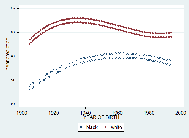
The graph has the following pattern :
The attentive reader will ask. Why using numbers as far as 8 or 9 digits after the decimal point ? Well, the problem is that with squared and cubic terms, even a small value is important. We shouldn't stop at 2 or 3 digits after the decimal.
Now, let's explain the calculation. What does it mean to do Yhat = intercept + coeff*var1 ? Let's say we have a sample of 10 individuals. Each of them having different values in all variables. And let's use a simpler model.
Yhat(wordsum) = intercept + coeff(bw1) + coeff(cohortc) + coeff(bw1cohortc)
In this model, I obtained an intercept of 4.8957, and coefficients of 1.369, 0.00808, and -0.01537. Now, let's look at our data.
The Yhat column above is the Yhat requested directly from the software, not computed by hand. Look closely at the first row. This individual has a value of 1 for bw1, cohortc and bw1cohortc. Then, his Yhat(wordsum) is given by :
Yhat1 = 4.8957+ 1.369*1 + 0.00808*1 + -0.01537*1
We do the same for the 9 remaining rows :
Yhat2 = 4.8957+ 1.369*1 + 0.00808*-19 + -0.01537*-19
Yhat3 = 4.8957+ 1.369*1 + 0.00808*-47 + -0.01537*-47
Yhat4 = 4.8957+ 1.369*1 + 0.00808*-36 + -0.01537*-36
Yhat5 = 4.8957+ 1.369*1 + 0.00808*-8 + -0.01537*-8
Yhat6 = 4.8957+ 1.369*1 + 0.00808*-26 + -0.01537*-26
Yhat7 = 4.8957+ 1.369*1 + 0.00808*-45 + -0.01537*-45
Yhat8 = 4.8957+ 1.369*1 + 0.00808*-29 + -0.01537*-29
Yhat9 = 4.8957+ 1.369*1 + 0.00808*-32 + -0.01537*-32
Yhat10 = 4.8957+ 1.369*0 + 0.00808*-5 + -0.01537*0
And we get our Yhat column :
6.25741
6.40321
6.60733
6.52714
6.32302
6.45424
6.59275
6.47611
6.49798
4.85530
You see the values are close to the ones displayed in my data window. But not exactly the same, due to rounding bias. Still, the calculation of Yhat is straightforward. If we want to control for covariates such as SES variables, things will become tedious. Let's add in our regression the variable gender. We get this graph.
regress wordsum bw1 cohortc cohortc2 cohortc3 bw1cohortc bw1cohortc2 bw1cohortc3 gender [pweight = weight], beta
predict pred2 if e(sample), xb
graph twoway (scatter pred2 cohort if bw1==0, msymbol(Oh)) (scatter pred2 cohort if bw1==1, msymbol(O)), legend(label(1 black) label(2 white))
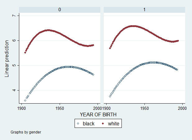
Ok... what's happening... ? If you haven't guessed yet, the answer is given in the following graph.
graph twoway (scatter pred2 cohort if bw1==0, msymbol(Oh)) (scatter pred2 cohort if bw1==1, msymbol(O)), by(gender) legend(label(1 black) label(2 white))
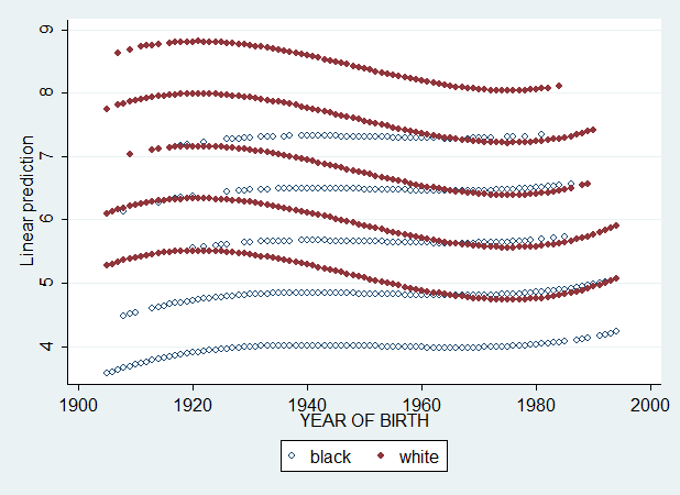
This is a graph of Yhat vs cohort by gender values (0=male, 1=female). Now, imagine we use degree (mean-centered) variable instead of gender. Since degree has 5 values, we should get 5 curves for whites and 5 curves for blacks. Let's see...
regress wordsum bw1 cohortc cohortc2 cohortc3 bw1cohortc bw1cohortc2 bw1cohortc3 degreec [pweight = weight], beta
predict pred3 if e(sample), xb
graph twoway (scatter pred3 cohort if bw1==0, msymbol(Oh)) (scatter pred3 cohort if bw1==1, msymbol(O)), legend(label(1 black) label(2 white))
Exactly as I said. And now let's see what happens if I also add degree, educ, logincome and age, age^2 and age^3 (all mean-centered).
regress wordsum bw1 cohortc cohortc2 cohortc3 bw1cohortc bw1cohortc2 bw1cohortc3 degreec educc logincomec agec agec2 agec3 [pweight = weight], beta
predict pred4 if e(sample), xb
graph twoway (scatter pred4 cohort if bw1==0, msymbol(Oh)) (scatter pred4 cohort if bw1==1, msymbol(O)), legend(label(1 black) label(2 white))
No. It's impossible to read. And we want to ask. How can we get a reliable curve when plotting Yhat ? Requesting the Yhat from the software appears difficult. If you haven't guessed yet, we can do it by just ignoring the SES variables in our calculation of Yhat. After all, the regression coefficients for bw1, cohortc, cohortc2, cohortc3, bw1cohortc, bw1cohortc2, bw1cohortc2, are the mean predicted values for these respective variables when degree, educ, logincome and age are held constant. So, Yhat should be computed simply as follows :
Yhat = intercept + coeff(bw1) + coeff(cohortc) + coeff(cohortc2) + coeff(cohortc3) + coeff(bw1cohortc) + coeff(bw1cohortc2) + coeff(bw1cohortc3)
In Stata, we do :
regress wordsum bw1 cohortc cohortc2 cohortc3 bw1cohortc bw1cohortc2 bw1cohortc3 agec agec2 agec3 logincomec educc degreec [pweight = weight], beta
gen pred5 = 5.251754 + 0.9560995*bw1 + -0.0044371*cohortc + 0.0003048*cohortc2 + 0.00000222*cohortc3 + -0.0141784*bw1cohortc + -0.000096*bw1cohortc2 + 0.00000426*bw1cohortc3
label variable pred5 "Predicted Wordsum scores"
graph twoway (scatter pred5 cohort if bw1==0, msymbol(Oh)) (scatter pred5 cohort if bw1==1, msymbol(O)), legend(label(1 black) label(2 white))
In SPSS, we do :
REGRESSION
/MISSING LISTWISE
/STATISTICS COEFF OUTS CI(95) R ANOVA COLLIN TOL CHANGE ZPP
/CRITERIA=PIN(.05) POUT(.10)
/NOORIGIN
/DEPENDENT wordsum
/METHOD=ENTER bw1 cohortc cohortc2 cohortc3 bw1cohortc bw1cohortc2 bw1cohortc3 agec agec2 agec3 logincomec educc degreec
/SAVE PRED ZPRED.
COMPUTE pred2 = 5.251754 + 0.9560995*bw1 + -0.0044371*cohortc + 0.0003048*cohortc2 + 0.00000222*cohortc3 + -0.0141784*bw1cohortc + -0.000096*bw1cohortc2 + 0.00000426*bw1cohortc3.
GRAPH
/SCATTERPLOT(BIVAR)=cohort WITH pred2 BY bw1
/MISSING=LISTWISE
/SUBTITLE='Wordsum score across cohort by race'.
And we get the following graph :
That graph is nice. We see, again, that the black-white difference has been halved.
Before closing this section, I want to say there is another way to use regression. By means of dummy variables. They are good substitutes for non-linear terms. The drawback is that the range of values assigned to each dummies can be arbitrary. In my situation, it is, but only because I wanted to avoid low sample sizes in the lowest and highest values of my dummy variables. The advantage is that we do not need to have the raw data set to make predictions. Dummy variables are coded as 0 and 1. So, multiplication of a coefficient by a variable is not needed. In dummy variable regression, we need to drop one dummy, in order to avoid perfect collinearity among the variables.
Let's say I want to do this in Stata :
regress wordsum bw1 cohortdummy2 cohortdummy3 cohortdummy4 cohortdummy5 cohortdummy6 bw1C2 bw1C3 bw1C4 bw1C5 bw1C6 aged1 aged2 aged3 aged4 aged6 aged7 aged8 aged9 bw1aged1 bw1aged2 bw1aged3 bw1aged4 bw1aged6 bw1aged7 bw1aged8 bw1aged9 gender [pweight = weight], beta
(sum of wgt is   2.2641e+04)
Linear regression                                      Number of obs =   22156
                                                       F( 28, 22127) =   60.61
                                                       Prob > F      =  0.0000
                                                       R-squared     =  0.0771
                                                       Root MSE      =  1.9883
------------------------------------------------------------------------------
             |               Robust
     wordsum |      Coef.   Std. Err.      t    P>|t|                     Beta
-------------+----------------------------------------------------------------
         bw1 |   1.595729   .2327211     6.86   0.000                 .2596706
cohortdummy2 |   .1981999   .1929249     1.03   0.304                 .0377756
cohortdummy3 |    .761507    .203674     3.74   0.000                 .1544235
cohortdummy4 |   .4735792   .2105816     2.25   0.025                 .0936345
cohortdummy5 |   .7437521    .220181     3.38   0.001                 .1325745
cohortdummy6 |   .9899584    .239162     4.14   0.000                 .1359903
       bw1C2 |  -.0381255   .2043839    -0.19   0.852                -.0069422
       bw1C3 |  -.2907772   .2153527    -1.35   0.177                 -.056325
       bw1C4 |  -.2392785   .2238821    -1.07   0.285                -.0447022
       bw1C5 |  -.5866855   .2348553    -2.50   0.012                -.0974284
       bw1C6 |  -.5478369   .2568472    -2.13   0.033                -.0683153
       aged1 |  -.8548259   .1565771    -5.46   0.000                -.1330508
       aged2 |   -.478698   .1470472    -3.26   0.001                -.0759053
       aged3 |  -.1870506   .1448449    -1.29   0.197                -.0287963
       aged4 |  -.0239464   .1466968    -0.16   0.870                -.0037029
       aged6 |  -.1941283   .1513518    -1.28   0.200                -.0307706
       aged7 |   .0849586   .1652006     0.51   0.607                 .0126335
       aged8 |  -.1892286   .1887384    -1.00   0.316                -.0261891
       aged9 |  -.4979676   .2521138    -1.98   0.048                -.0658842
    bw1aged1 |  -.0730532   .1722452    -0.42   0.671                -.0105926
    bw1aged2 |   .0240677   .1609454     0.15   0.881                 .0035682
    bw1aged3 |  -.0830173   .1586071    -0.52   0.601                -.0118999
    bw1aged4 |  -.0142871   .1585825    -0.09   0.928                -.0020842
    bw1aged6 |   .2693492   .1650585     1.63   0.103                 .0401329
    bw1aged7 |  -.0761591   .1801369    -0.42   0.672                -.0106595
    bw1aged8 |   .3038935   .2034854     1.49   0.135                 .0400347
    bw1aged9 |   .5817023   .2653968     2.19   0.028                 .0736105
      gender |   .1698627   .0298917     5.68   0.000                 .0408736
       _cons |   4.506666   .2194024    20.54   0.000                        .
------------------------------------------------------------------------------
The corresponding syntax in SPSS being :
REGRESSION
/MISSING LISTWISE
/STATISTICS COEFF OUTS CI(95) R ANOVA COLLIN TOL CHANGE ZPP
/CRITERIA=PIN(.05) POUT(.10)
/NOORIGIN
/DEPENDENT wordsum
/METHOD=ENTER bw1 cohortdummy2 cohortdummy3 cohortdummy4 cohortdummy5 cohortdummy6 bw1C2 bw1C3 bw1C4 bw1C5 bw1C6 aged1 aged2 aged3 aged4 aged6 aged7 aged8 aged9 bw1aged1 bw1aged2 bw1aged3 bw1aged4 bw1aged6 bw1aged7 bw1aged8 bw1aged9 gender
/SAVE PRED ZPRED.
My intercept is 4.506666. And the coefficient for bw1 is 1.595729. What are these values ? Since cohortdummy1 and bw1C1 are missing (reference categories), and the intercept being the value of Y when all X are zero, thus the intercept is the black score for cohortdummy1. And bw1 is the black-white difference net of the influence of all other X variables. So, bw1 is effectively bw1C1. We get the following columns :
4.507   0   1
4.705   0   2
5.268   0   3
4.980   0   4
5.250   0   5
5.497   0   6
6.102   1   1
6.262   1   2
6.573   1   3
6.337   1   4
6.259   1   5
6.545   1   6
In the first column, the first six rows are the black scores (intercept, intercept+cohortdummy2, intercept+cohortdummy3, etc.), the last six rows are the white scores (intercept+bw1, intercept+bw1+cohortdummy2+bw1C2, intercept+bw1+cohortdummy3+bw1C3, etc.), the second column is the racial category (black=0, white=1) and the third column is the category of the cohort dummy variables.
If we plot Yhat against cohort by race category, we get this :
clear
twoway (scatter var1 var3, msymbol(O) jitter(0)) (lfit var1 var3 if var2==0) (lfit var1 var3 if var2==1), ytitle(predicted wordsum) legend(order(2 "black" 3 "white"))
Again, a black-white convergence in Wordsum.
Logistic regression
The method is similar to OLS regression, except that the intercept is a logit. And a logit is not a probability. So, to obtain that probability, we exponentiate the logit, and we obtain the odds. Finally, we get the probability by computing odds/(1+odds).
Here, I have the opportunity to introduce to the so-called Differential Item Functioning (DIF) methods. The idea in the different kinds of DIF techniques is similar. We want to know if the group variable contribute to the probability of correct response in any given item when the total score (sum of all items) is included as regressor. DIF methods are complicated, so I will shorten the description of LR method.
In logistic regression (LR), we have typically three models. One involves only total score, the second adds group variable, the third adds the interaction of group with total score. The first model can be regarded as the Rasch model which makes the assumption of unidimensionality (i.e., only the total score accounts for the variation in the probabilities of correct response). The second model is aimed to detect uniform DIF. The third model is aimed to detect non-uniform DIF. If we want a measure of "effect size" for the model with both uniform and non-uniform DIF, we calculate the difference in R² between model 1 and model 3. But I would rather use its square root. A better, simpler method consists in plotting the probabilities, or Item Characteristic Curves (ICC). Plotting the ICC in model 3 gives both forms of DIF. So, we will disregard R² and look at the ICC. I select word g as the dependent variable because it is by far the most biased item among all of them. The interested reader can try other items.
In Stata, the syntax is :
logit wordg wordsum bw1 bw1wordsum [pweight = weight]
predict logit if e(sample), xb
gen logit1 = -4.101398 + 0.4641457*wordsum + -2.904372*bw1 + 0.4882717*bw1wordsum
gen odds1 = exp(logit1)
gen probability1 = odds1/(1+odds1)
graph twoway (scatter probability1 wordsum if bw1==0, msymbol(Oh)) (scatter probability1 wordsum if bw1==1, msymbol(O)), legend(label(1 black) label(2 white))
In SPSS, the syntax is :
LOGISTIC REGRESSION VARIABLES wordg
/METHOD=ENTER wordsum
/METHOD=ENTER bw1
/METHOD=ENTER bw1wordsum
/SAVE=PRED
/CLASSPLOT
/PRINT=GOODFIT CI(95)
/CRITERIA=PIN(0.05) POUT(0.10) ITERATE(20) CUT(0.5).
compute logit1 = -4.101398 + 0.4641457*wordsum + -2.904372*bw1 + 0.4882717*bw1wordsum.
compute odds1 = exp(logit1).
compute probability1 = odds1/(1+odds1).
execute.
GRAPH
/SCATTERPLOT(BIVAR)=wordsum WITH probability1 BY bw1
/MISSING=LISTWISE
/SUBTITLE='Probability of correct response'.
I calculate the logit and probabilities manually, but we can ask the software to do it for us.
The probability of correct answer in word g is clearly different between blacks and whites. Of course, this is not all. We need to know if the black-white difference in the TCC or total characteristic curve (i.e., the sum of all ICCs) differs from the black-white difference in the raw wordsum score. We need also to answer whether the DIF methods really require that (almost) all items should be DIF free or not. And if these DIFs introduce biases in prediction (Roznowski & Reith, 1999). These are all complex questions, and I have planned to answer them in a forthcoming article.
Multilevel (linear mixed-effects) regression
Multilevel regression is exceedingly complex, and probably no less complex than SEM, MGCFA and IRT. If you need a description, go read my paper. Then, I will be using a 2-level model. In the fixed (level-1) component, I have bw1, aged1-aged9 dummies and the interaction of bw1 with aged1-aged9 dummy variables. The fixed portion can be compared to the classical OLS regression. The random (level-2) component includes cohort21 as random intercept and bw1 as random slope. These variables are in fact residuals of their respective fixed coefficients. That is, a random coefficient is estimated for each of the 21 categories of my cohort21 and these coefficients are the variations around the model mean intercept estimated in the fixed component. And bw1 random slope will also have 21 random coefficients because this random slope is specified to vary across each value of the cohort21 variable. The random coefficients in the random slope bw1 are the variations around the average fixed slope bw1 estimated in the fixed component of the multilevel model.
By holding constant age, and letting cohort vary in the population, we are able to break the linear dependency between age and cohort, i.e., separate the effect of age from the effect of cohort with respect to black-white score gap. This is important because, as we have seen, the black-white gap increases with age, decreases with cohort. But age decreases in more recent cohorts. There is a potential confounding here that classical regression cannot disentangle because it assumes that the effects of all X variables are additive (see Yang & Land, 2008, p. 322).
In this kind of analysis, there are two ways of making graphs.
The first is to use the estimated random coefficients of the intercept and slope (in the case your model involves a random slope model). Since the intercept is the value of Y for all Xs=0, the random effects of cohort are in fact the random variation of black scores over time. And since the random slope is the dichotomized race variable, the variation in white score over time can be obtained by adding the random coefficients of cohort to the respective random coefficients of the random slope bw1. We now obtain two columns (i.e., vectors) of values and we can plot them by group (race and cohort) categories.
The second is more straightforward. It simply requires to compute the fitted values, and all softwares can automatically request the fitted (predicted) Y. But in multilevel regression, the fitted values are the sum of the fixed component and the random component. Usually, the softwares should be able to request either the fitted, or the fixed effects, or the random effects (EBLUPs) predictors.
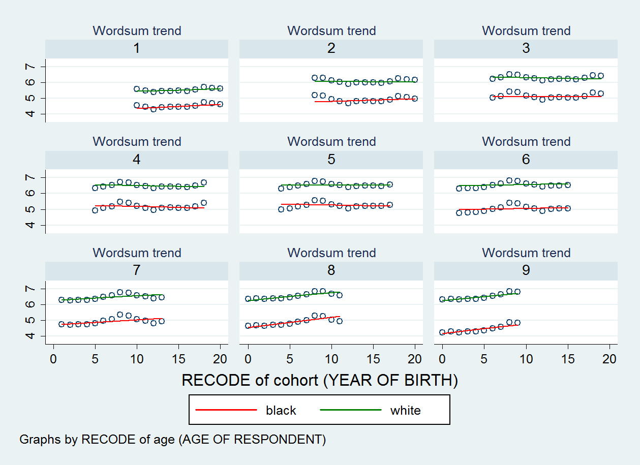
To the extent I have included many variables (nine age dummies and a race dichotomy), a simple scatter of the fitted wordsum against cohort21 will show variations of data points corresponding to the fixed effects of age and race. A possibility is to graph the scatter for each value of the age dummy. So, here, I request a series of scatter plot by age.
The syntax in Stata is :
xtmixed wordsum bw1 aged1 aged2 aged3 aged4 aged6 aged7 aged8 aged9 bw1aged1 bw1aged2 bw1aged3 bw1aged4 bw1aged6 bw1aged7 bw1aged8 bw1aged9 || cohort21: bw1, reml cov(un) var
predict xtfitted3 if e(sample), fitted
twoway (scatter xtfitted3 cohort21, msymbol(Oh) jitter(0)) (lfit xtfitted3 cohort21 if bw1==0, lcolor(red)) (lfit xtfitted3 cohort21 if bw1==1, lcolor(green)), by(age9) legend(cols(4) size(small)) title("Wordsum trend", size(medsmall)) legend(order(2 "black" 3 "white"))
The syntax in SPSS is :
WEIGHT OFF.
MIXED wordsum WITH bw1 aged1 aged2 aged3 aged4 aged6 aged7 aged8 aged9 bw1aged1 bw1aged2 bw1aged3 bw1aged4 bw1aged6 bw1aged7 bw1aged8 bw1aged9
/CRITERIA=CIN(95) MXITER(100) MXSTEP(10) SCORING(1) SINGULAR(0.000000000001) HCONVERGE(0, ABSOLUTE) LCONVERGE(0, ABSOLUTE) PCONVERGE(0.000001, ABSOLUTE)
/FIXED=bw1 aged1 aged2 aged3 aged4 aged6 aged7 aged8 aged9 bw1aged1 bw1aged2 bw1aged3 bw1aged4 bw1aged6 bw1aged7 bw1aged8 bw1aged9 | SSTYPE(3)
/METHOD=REML
/PRINT=SOLUTION TESTCOV
/RANDOM=INTERCEPT bw1 | SUBJECT(cohort21) COVTYPE(UN)
/SAVE=FIXPRED PRED RESID.
GRAPH
/SCATTERPLOT(BIVAR)=cohort21 WITH PRED_1 BY bw1
/PANEL ROWVAR=age9 ROWOP=CROSS
/MISSING=LISTWISE.
GRAPH
/LINE(MULTIPLE)=MEAN(PRED_1) BY cohort21 BY bw1
/PANEL ROWVAR=age9 ROWOP=CROSS.
SORT CASES BY age9.
SPLIT FILE LAYERED BY age9.
GRAPH
/SCATTERPLOT(BIVAR)=cohort21 WITH PRED_1 BY bw1
/MISSING=LISTWISE.
If you find the SPSS syntax a little bit complex, you should definitely read Bickel's (2007, p. 113) guide. In SPSS, it seems difficult to request a multi-panel plot. I use Stata again :
Here, we don't see the black-white score gap narrowing. So, what happened ? Oh. Nothing fishy. It's a question of which method is the most adequate. I have answered this question in my paper. But if the explanation is not simple enough, I will make it even simpler in my forthcoming article on multilevel models.

