IQ Regression to the Mean : the Genetic Prediction Vindicated

The IQ differences between blacks and whites lead to differences in sibling regression to the mean. The races regress to different means. Criticisms were made ​​about the hereditarian interpretation of the differential sibling regressions. I will demonstrate that this phenomenon (1) is not a statistical artifact and (2) is consistent with the hereditarian interpretation of it.

Introduction. Although regression to the mean is sometimes interpreted as a strong support for the hereditarian hypothesis with regard to the nature of the black-white IQ difference (Jensen, 1973, pp. 110-119; 1998, pp. 468-472; Rushton & Jensen, 2005, p. 263), others suggest that this phenomenon fails to narrow the race-IQ debate.

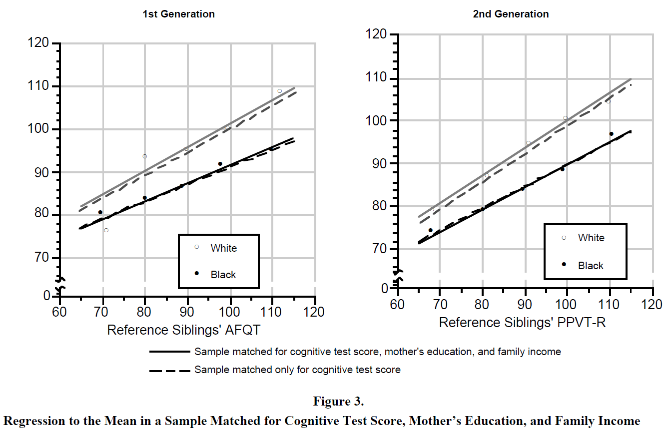
The hereditarians argued that regression occurs because parents and children share 50% of their genes, this phenomenon is simply reflecting the non-transmission of heritable traits (that is, they are not shared). The degree of regression increases when the degree of kinship decreases. Environmentalists, however, believe that regression to the mean can also be understood in terms of differences in culture or environment. Racial differences regarding sibling regression to the mean could be interpreted as a between-family difference, insofar as black and white siblings with equal IQs do not necessarily have the same home environment quality. After all, environmentalists may argue that black parents will provide a poor cognitive environment to their children, even if black and white parents were perfectly matched for IQ. But if the environmental theory of race differences is really tenable, we should expect a convergence in differential sibling regression to the mean. Any other result purely contradicts this theory.

Another kind of criticism (Kaplan, 2001, p. 16-18; Neuroskeptic, 2010) focuses on the interpretation of the regression to the mean per se. It was suggested that this phenomenon is just a statistical artifact. An example may help to understand the argument. Suppose in the next month, the number of car accidents in the country will suddenly double. The government responds by placing additional cameras, strengthening surveillance systems. This strategy will fail because in the next month, the number of accidents will go back to its initial level. Regression to the mean. In other words, the regression is thought to be a cyclical phenomenon of whatever luck and chance.

But that's not clear at all. What kind of luck explains the fact that the children of high-IQ parents have lower IQs while they are reared in cognitive stimulating environments, when the children of low-IQ parents who were raised in chaotic environments still have higher IQs than their parents ? The IQs regress halfway (50%) to the population mean at both sides of the IQ distribution. If we stick to the Dickens-Flynn model (2001) of feedback loops, one would expect that children of high-IQ parents have higher IQ and children of low-IQ parents an IQ even lower. But the opposite happens. This criticism, in the end, does not provide any explanation for the fact that the regression is homogeneous across the different levels of IQ. As Jensen made it clear, the IQ subgroups do not depart from linearity for an IQ range going from 50 to 150.

While some say that regression to the mean occurs because of some kind of (random) measurement errors, it should be noted that IQ regression to the mean analyses are usually performed by using the method of estimated true scores, that is, IQ scores corrected for measurement error, or unreliability, with the formula :

Tˆ = rXX′ (X − MX) + MX

where Tˆ is the estimated true score, X the observed score, rXX′ the reliability coefficient of the test, and MX being the mean of the group. Why this method reduces the "luck" factor has been explained in Bias in Mental Testing (1980, pp. 276-277) by Jensen himself :

The net effect of using such estimated true scores, besides increasing the accuracy of measurement, is to reduce the higher scores of persons belonging to low-scoring subgroups and boost the lower scores of persons belonging to high-scoring subgroups. Such an outcome may seem unfair from the standpoint of members of the lower-scoring subgroups, but it is merely the statistically inevitable effect of increasing the accuracy of measurement. When higher scores are preferred in the selection procedure, the “luck” factor resulting from unreliability statistically favors persons belonging to lower-scoring groups. The “luck” factor is minimized by using estimated true scores instead of obtained scores.

[...] If test reliability is quite high (i.e., above .90), however, the slight gains in accuracy and predictive validity from using estimated true scores may hardly repay the extra computational effort.

But given that the reliability of AFQT is about 0.95 (Winship & Korenman, 1999), this method will leave the results unaffected in any case.

Still another critique, from Mackenzie (1984, p. 1220) this time, made the case that blacks and whites will regress to the same mean if the parent-child correlations or sibling correlations were calculated from pooled samples of blacks and whites. Of course, this tells us nothing about the causes of the racial differences in sibling regressions. Because, on the contrary, when the levels of IQ increase, the racial differences in sibling regressions will tend to converge, according to the environmental hypothesis. If this is not the case, the environmental interpretation is untenable. This was exactly what Jensen (1973) wanted to know : if one of the IQ subgroups at both ends shows some deviations from linearity. Or stated differently, to see if the regression lines converge at higher levels of IQ.

But the fact that the black-white IQ difference increases with SES levels (Jensen, 1973, pp. 241-242; Herrnstein & Murray, 1994, pp. 287-288; Jensen, 1998, p. 358; Gottfredson, 2003, Table 2; Hu, Oct.20.2013, Jan.18.2013) is hardly explainable from the environmental standpoint. Thus, Jensen (1973, p. 119) believed that it could be easily explained by the BW difference with regard to sibling regression toward the mean.

Method and Data. NLSY79 and NLSY97 were used for the present analysis, because sibling data and IQ subtests were available. Factor analysis can be performed for extracting g (analysis #1) and Jensen's method of correlated vectors can be used for testing the association between sibling correlations on ASVAB subtests and black-white gaps as well as g-loadings in those subtests (analysis #2).

If one wants to replicate the present finding using my syntax and variables for NLSY79 (here) and NLSY97 (here), recall that SPSS is needed. Creating a free NLS Investigator account is needed if we wish to collect the relevant variables. Then, do a quick search by terms, keywords, as shown below :

Then, download your collection of selected variables, and copy/paste the files into a new file. Before running the syntax page, recall that the handle file should look like this.

Regarding the differential sibling regression to the mean, the purpose was to replicate and extend further Murray's analysis on the NLSY79. I recoded the key variable as follows : BHW=1 for blacks, BHW=2 for hispanics, BHW=3 for whites, SIBLING=1 for full siblings, SIBLING=2 for unrelated and half siblings. Thanks to the CASESTOVARS command, it was possible to identify the NLSY full siblings. This command breaks a variable into a certain number of categories (depending on the number of values of this variable). So, when a variable ended with an .1 or an .2, this was the numero of the identified sibling : .1 for sibling #1 and .2 for sibling #2. The numbers after the sign "=" designate the categories of my dummy variables.

But because I was unable to find a magical SPSS syntax, I have to delete the missing values manually. The easiest way to do this hopefully is to simply use the "Sort Ascending" option in the SPSS data editor page for the relevant column. This will list the empty cells first. So I use this option for deleting missing values among siblings #1 and then among siblings #2. ("Copy Dataset" is a very useful function that duplicates the data window if some cases have been deleted by error)

Of course, some anomalies have been detected. For example, when one sibling self-identified as black or hispanic and the other sibling self-identified as white, and both responded that they are full siblings. These cases are deleted. Similarly, even when both agreed about their racial identification, sometimes the first sibling said the other one is a full sibling while this second sibling said the other one is not a full sibling. These cases, too, are deleted. Here's an example of anomaly :

Also, there should be no missing values in either SIBLING.1 or SIBLING.2. Missing values in BHW (my race variable) is of no concern when both siblings said they are not full siblings. But if they were full siblings, empty values of BHW pose a problem because of the way I coded BHW, empty values are the respondents who are not either blacks, hispanics or whites. Those cases are deleted. For doing this, use Sort Ascending option on SIBLING.1 and SIBLING.2 columns. Values of 1 are listed first. Then re-use this option on the BHW column. This will put at the top of the list the full siblings who have empty values in BHW (in other words, full siblings who are not either blacks, whites or hispanics).

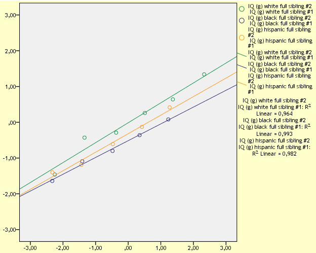
Because the data points are scattered everywhere when performing an overlay scatter plot (with option 'Exclude cases variable by variable') in order to display the regression lines for each racial group, I also display a graph with IQ subgroups, as Murray (1999) did :

To do this with the appropriate SPSS syntax (here), I categorized the IQs of siblings #1 for each race by averaging the IQs of all same-race subjects that have an IQ between -3 SD and -2 SD below the mean of the full sample analyzed, and IQ between -2 SD and -1 SD below the mean, and so forth. Filters and comparisons of means were used for this purpose.

Because Wordpress doesn't allow SPSS file, you have to send me a mail, if you want it. Hopefully, Wordpress allows Excel file to be uploaded. If you don't have Excel however, Kingsoft Spreadsheets is a good alternative.

NLSY79 g factor MCV regression to the mean and sibling correlations
NLSY97 g factor MCV regression to the mean and sibling correlations

I also assembled the data from half and unrelated siblings but I haven't reported the result here because I found it uninformative (range of restriction of cognitive abilities, small sample size, ...).

Results. The first analysis compares the BW sibling regression lines in the g dimension and non-g dimension of cognitive tests. The second analysis aims to replicate Jensen's findings using his method of correlated vectors.

Analysis 1. The (PAF) factor analysis of the NLSY (97 and 79) ASVAB subtests allows the extraction of a g-factor score and a non-g factor score, represented by the loadings in the first factor and the second factor in the factor matrix. The interest is to see whether or not the degree of regression toward the mean is changing accordingly from the g dimension to the non-g dimension of cognitive tests.

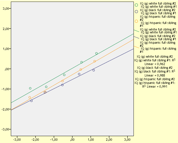
Here, I display a graph showing the sibling regression without grouping IQs and another graph with IQ subgroups. The advantage of the latter, as stated above, is to have a better look at any deviation from linearity, as Murray did. Here's what the NLSY97 sibling regressions look like :

The x axis (horizontal, from left to right) shows the IQs of sibling #1. The y (vertical) axis shows the IQs of sibling #2. As we can see, there is no convergence in the regression lines at higher levels of IQ. The BW sibling gap may appear even larger. The BW sibling difference is about 0.50 SD.

Above are the graphs showing the sibling regression lines for the NLSY79. Here again, we see no convergence in the g-factor dimension. The hispanic line falls once again between the black and white lines.

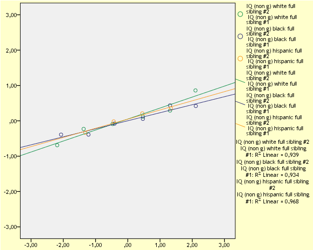
Consistent with Murray (1999) and Jensen (1973), none of the above data points representing the IQ subgroups show any deviation from linearity. Now, let's look at the non-g factor dimension, first for the NLSY97 and then for the NLSY79 :

Regarding the R² values for IQ subgroups, we shouldn't put much faith on them. It's obvious that they are totally uninformative here. What is of significance here is that the racial sibling gap is trivial. The IQs of siblings #2 move just slightly (-0.5 SD to +0.5 SD) as the IQs of sibling #1 are changing (-2 SD to +2 SD).

If the degree of regression is a function of the g-loadedness of IQ tests, with more regression among the less heritable component of IQ tests, it is hard to believe that this phenomenon is a mere statistical artifact. Next analysis provides another test of this assumption.

Analysis 2. Now we test Jensen's predictions. In The g Factor (pp. 471-472), he wrote :

A number of different mental tests besides IQ were also given to the pupils in the school district described above. They included sixteen age-normed measures of scholastic achievement in language and arithmetic skills, short-term memory, and a speeded paper-and-pencil psychomotor test that mainly reflects effort or motivation in the testing situation. [50] Sibling intraclass correlations were obtained on each of the sixteen tests. IQ, being the most g loaded of all the tests, had the largest sibling correlation. All sixteen of the sibling correlations, however, fell below +.50 to varying degrees; the correlations ranged from .10 to .45., averaging .30 for whites and .28 for blacks. (For comparison, the average age-adjusted sibling correlations for height and weight in this sample were .44 and .38, respectively.) Deviations of these sibling correlations from the genetic correlation of .50 are an indication that the test score variances do reflect nongenetic factors to varying degrees. Conversely, the closer the obtained sibling correlation approaches the expected genetic correlation of .50, the larger its genetic component. These data, therefore, allow two predictions, which, if borne out, would be consistent with the default hypothesis:

1. The varying magnitudes of the sibling correlations on the sixteen diverse tests in blacks and whites should be positively correlated. In fact, the correlation between the vector of sixteen black sibling correlations and the corresponding vector of sixteen white sibling correlations was r = +.71, p = .002.

2. For both blacks and whites, there should be a positive correlation between (a) the magnitudes of the sibling correlations on the sixteen tests and (b) the magnitudes of the standardized mean W-B differences (average difference = 1.03σ) on the sixteen tests. The results show that the correlation between the standardized mean W-B differences on the sixteen tests and the siblings correlations is r = +.61, p < .013 for blacks, and r = +.80, p < .001 for whites.

Note that with regard to the second prediction, a purely environmental hypothesis of the mean W-B differences would predict a negative correlation between the magnitudes of the sibling correlations and the magnitudes of the mean W-B differences. The results in fact showing a strong positive correlation contradict this purely nongenetic hypothesis.

To recall, the default hypothesis (Jensen, 1998, p. 448) posits that the genetic and the environmental factors that cause the between-groups difference exist within each group (but not necessarily in equal degrees).

First of all, let's see what the relationship between the vector of sibling correlations and the vector of g-loadings looks like. In the NLSY97, the BW g-loadings correlate strongly with white sibling correlations (+0.80) and black sibling correlations (+0.90). The HW g-loadings also displayed a strong relationship with both white and hispanic sibling correlations (+0.80). And again, the BH g-loadings also show a strong positive correlation with hispanic and black sibling correlations (respectively, +0.90 and +0.80). In the NLSY79, BW g-loadings correlate with sibling correlations for whites at about +0.80 and for blacks around +0.35 and +0.15. The HW g-loadings correlate strongly with white sibling correlations (around +0.75) and with hispanic sibling correlations (around +0.75). What is unexpected is that BH g-loadings correlate negatively with sibling correlations for blacks (around -0.20) and for hispanics (about -0.30 and -0.50).

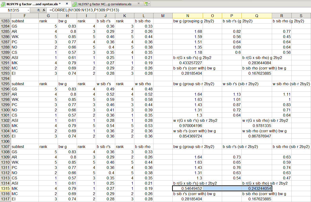
Another method (apparently suggested by Bartholomew, 2004) that might improve the reliability of estimates consists in grouping two by two the subtest g-loadings and/or sibling correlations, by order/rank of estimates. For example, if GS and AR subtests have the two highest loadings, we first average the g-loadings of GS and AR, and then average the sibling correlations of GS and AR, and we repeat the process for the two next highest loadings, and so forth. But we can also group by d gaps, by averaging the two highest d gaps, and repeating the process for the second two highest d gaps, and so on, and finally by averaging the corresponding g-loadings in the column vector. And as the above picture shows, the correlation between the magnitude of BW g-loadings and the black sibling correlations is a little bit higher (+0.43 and +0.28, if we use g grouping; or +0.55 and +0.24 if we use sib r's grouping).

Generally speaking, this finding supports the view that the magnitude of sibling regressions toward the mean diminishes as the g-loadedness of the test increases, which is also consistent with Analysis #1.

But what about the (non-g) loadings of the second factor with sibling correlations ? In the NLSY97, these associations are usually negative and none of them showed a positive slope for all races. In the NLSY79, however, the white full sibling correlations were strongly and positively associated (r and rho) with non-g loadings for BW non g-loadings, but this relationship is much smaller for HW non g-loadings. Among blacks, this relationship is positive but much smaller and looks like a random dispersion of dots for BW non g-loadings, or is near zero for BH non g-loadings. Among hispanics, they were small negative or small positive.

Now, regarding Jensen's first prediction, the NLSY97 shows a very strong positive correlation between the vector of white sibling correlations and the vector of black sibling correlations (around +0.80 and +0.90). Between hispanics and whites, the correlations were also very high (around +0.90). Between hispanics and blacks, the correlations were about +0.80 and +0.90. In the NLSY79 I found a moderate positive correlation between the vector of white sibling correlations and the vector of black sibling correlations (around +0.40). Between whites and hispanics, the correlations turned to be about +0.40 or +0.50. Between blacks and hispanics, the correlations were around +0.30.

Finally, with regard to Jensen's second prediction, the NLSY97 shows that the magnitude of the BW d gap is not related with the magnitude of black sibling correlations (near zero) or modestly with the white sibling correlations (around +0.20 or +0.15). The correlation between the HW d gap and sibling correlations is not trivial for whites (around +0.25 and +0.40) and for hispanics (around +0.40 and +0.50). Curiously, the correlation between BH d gap and sibling correlations is small for hispanics (around +0.10 and +0.15) but negative for blacks (-0.10 or -0.20). In the NLSY79, the magnitude of BW d gap correlates with black sibling correlations at about +0.10 and with white sibling correlations at about +0.05. The magnitude of HW d gap is positively correlated with sibling correlations for whites (around +0.40) and for hispanics (around +0.80 and +0.90). The magnitude of BH d gap shows a non-trivial negative relationship with sibling correlations for blacks (around -0.15 and -0.30) and for hispanics (around -0.25 and -0.50).

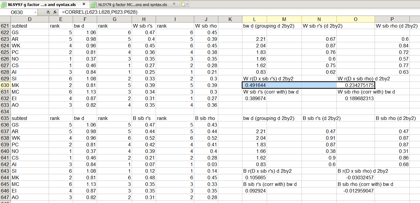
Using again Bartholomew's method, the correlation between the magnitude of BW d gap with white sibling correlations becomes a little bit higher (at about +0.49 for r's, and +0.23 for rho) while for black sibling correlations, it remains very low (+0.10 and -0.03, respectively) in the NLSY97. Regarding this, it should be noted that MCV totally failed to show a correlation between BW d gap and BW g-loadings in the NLSY97 even if there was in fact such a Spearman effect.

This method of course will not generate correlations as high as what Jensen found (about +0.60 and +0.80). But because none of these relationships were negative with regard to the black-white IQ gap, we can say that the environmental hypothesis is clearly rejected. Overall, my 2nd analysis attempting to replicate Jensen’s finding is mixed. It is not a great success, but it is not a failure either. The finding is still consistent with the hereditarian hypothesis but perhaps less than what he might have suggested.

Limitations. As explained above, regressed true scores were not used in analysis #1, but given the high reliability coefficient of AFQT (0.95), it will probably not affect the above result. Also, regarding the graphs of grouped IQs for g factor scores, the dots at both ends of the IQ distribution comprise in fact a very small sample size, with sometimes 10 or 20 sibling pairs.

Jensen's method of correlated vectors used in analysis #2 is not without critics (Dolan, 2000, p. 46; Dolan & Hamaker, 2001, pp. 16-19; Ashton & Lee, 2005, p. 438). Dolan is confident that MGCFA, rather than MCV, allows one to demonstrate that the g model fits better than the competing models, and at the same time, he says that Jensen's procedure provides no goodness of fit testing, with no test of B-W difference in covariance. Among other things, a hierarchical factor analysis (see Colom, 2002, for SPSS syntax) was not used as a secondary check of the existence of a general factor, and this poses a problem since Jensen (1998, pp. 96-97) has made it clear that hierarchical factor analysis could easily overcome the problem of what he calls a psychometric sampling error (that is, a situation where the extracted g is in fact a distorted g resulting from a biased representativeness of the tests in the test battery), although Ashton and Lee argued that its use does not overcome the many problems associated with a biased selection of subtests. On the other hand, Rushton (2007, p. 11) also defended the MCV. He made the case that the failure of Jensen's MCV can be due in fact to a biased criterion (i.e., dependent variable). In Bias in Mental Testing (1980, pp. 310, 383), Jensen indeed wrote the following :

A biased criterion is one that consistently overrates (or underrates) the criterial performance of the members of a particular subpopulation. A good example is sex bias in school grades: teachers generally give slightly higher grades to girls than to boys, even when the sexes are perfectly matched on objective measures of scholastic achievement.

When the criterion itself is questionable, we must look at the various construct validity criteria of test bias. If these show no significant amount of test bias, it is likely (although not formally proved) that the criterion, not the test, is biased. In a validity study, poor criterion measurement can make a good test look bad.

However, I don't see why this point should apply to the present analysis. But perhaps Jensen's MCV used in conjunction with meta-analyses along with further corrections for artifacts (sampling error, range restriction of g-loading vectors, perfect construct validity, ...) could yield a very promising results (te Nijenhuis, 2007, 2013; Joep Dragt, 2010).

Another significant difference between Jensen's application of MCV and mine, is that when he uses MCV to test the Spearman Hypothesis, his histogram (in, The g Factor, p. 382) shows a normal frequency distribution of g-loadings (g) and standardized mean B-W differences (d) for 149 subtests from 12 different test batteries (N = 286,901). But, in both the NLSY97 and NLSY79, it is clear that those distributions do not display normality in the frequency. As Jensen pointed out, a test of a Spearman effect using MCV should require, ideally, "large g loadings on the subtests and maximum variation among the subtests' g loadings; also, large mean group differences on the subtests and maximum variation among the group differences". So, this could be one of the reasons why the results from the MCV in Analysis #2 may appear sometimes contradictory.

If to be correctly applied, Jensen's MCV required a multitude of conditions, it appears that I haven't met those conditions in any case. If true, my findings related to the 2nd analysis must be considered with a pinch of salt.

Discussion. If, for reasons mentioned above, the BW sibling regression gap cannot be fully interpreted in terms of environments, we may think of a combination of genetic and shared environmental differences. But what kind of environment, exactly ? Chuck (Dec.8.2012), on “More thoughts on differential regression to the mean studies”, argues for a shared environmental effect, and Murray (1999) for a non-shared. Jensen (1973) seems to argue against shared environmental effects. In Educability & Group Differences, pp. 118-119, Jensen expresses his thoughts :

It can be claimed that though the white and Negro children are matched for IQ 120, they actually have different environments, with the Negro child, on the average, having the less intellectually stimulating environment. Therefore, it could be argued he actually has a higher genetic potential for intelligence than the environmentally favored white child with the same IQ. But if this were the case, why should not the Negro child’s siblings also have somewhat superior genetic potential? They have the same parents, and their degree of genetic resemblance, indicated by the theoretical genetic correlation among siblings, is presumably the same for Negroes and whites.

What Jensen has in mind would possibly be the idea that the absence of a convergence in the regression lines is difficult to explain in terms of differences in shared environment. But this would be true, also, with regard to non-shared environment. One cannot even begin to explain why blacks should be more environmentally depressed relative to whites at higher levels of IQ.